Gradient (그래디언트), Jacobian (자코비안) 및 Hessian (헤시안)

Calculus 관련 글 목차

• 참조 : https://gaussian37.github.io/math-mfml-multivariate_calculus_and_jacobian/
• 참조 : http://t-robotics.blogspot.com/2013/12/jacobian.html#.XGlnkegzaUk
• 참조 : https://suhak.tistory.com/944
• 참조 : https://gaussian37.github.io/math-mfml-multivariate_calculus_and_jacobian/

목차

• Gradient, Jacobian 및 Hessian의 비교 요약

• Gradient의 정의 및 예시

• Python을 이용한 Gradient 계산

• Jacobian의 정의 및 예시

• Python을 이용한 Jacobian 계산

• Hessian의 정의 및 예시

• Python을 이용한 Hessian 계산

Gradient, Jacobian 및 Hessian의 비교 요약

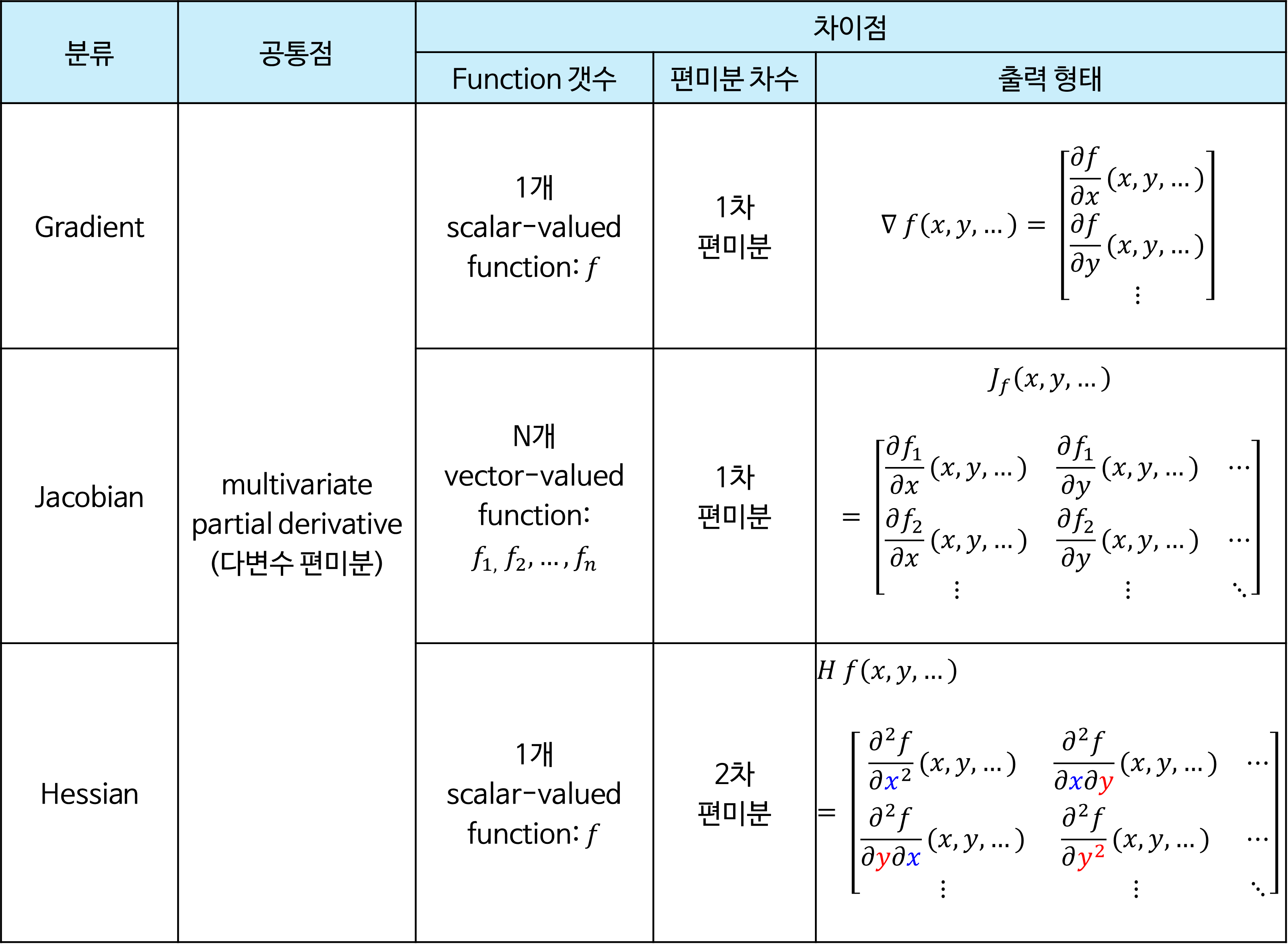
• 먼저 이번 글에서 다룰 3가지 개념인 Gradient, Jacobian, 그리고 Hessian의 내용을 간략하게 표로 정리하면 다음과 같습니다.

• 3가지 모두 Objective Function을 최적화할 때 사용한다는 점에서 다변수에 대한 편미분을 한다는 공통점이 있으나 알고리즘에 따라서 사용하는 값이 다르기 때문에 함수의 갯수, 편미분 차수에 차이점이 있습니다.
• 위 도표에서 보이는 것 처럼 Gradient는 1개의 함수에 대한 다변수 1차 편미분을 통해 벡터를 출력합니다. Jacobian은 Gradient를 확장하여 N개의 함수에 대한 다변수 1차 편미분을 통해 행렬을 출력합니다. 마지막으로 Hessian은 1개의 함수에 대한 다변수 2차 편미분을 통하여 행렬을 출력합니다. 2차 편미분을 거치기 때문에 편미분할 변수를 2가지 선택해야 하므로 2차원 행렬을 가지게 됩니다.
• 그러면 Gradient, Jacobian, Hessian의 개념과 실제 코드 상으로 어떻게 쉽게 구하는 지 살펴보도록 하겠습니다.
• 앞으로 사용할 용어 중 위 도표와 같이 단일 함수는 scalar-valued function이라고 하며 복수 개의 함수는 vector-valued function이라고 명명하곘습니다.

Gradient의 정의 및 예시

• scalar-valued multivariable function인 \(f(x, y, ...)\) 의 Gradient는 \(\nabla f\) 로 표기하며 그 의미는 다음과 같습니다.

• \[\nabla f = \begin{bmatrix} \frac{\partial f}{\partial x} \\ \frac{\partial f}{\partial y} \\ \vdots \end{bmatrix}\]

• 즉, 각 변수인 \((x, y, ...)\) 대하여 편미분한 결과를 벡터의 각 성분으로 가지는 것을 Gradient (Vectors)라고 합니다. 즉, 모든 변수를 고려한 변화량 (derivative)을 표현한 벡터가 됩니다. 따라서 Gradient는 scalar-valued multivariable function을 이용하여 vector-valued multivariable function을 만드는 연산이라고 말할 수 있습니다. 다음 예제들을 살펴보도록 하겠습니다.

• \[f(x, y) = x^{2} - xy\]
• \[\nabla f(x, y) = \begin{bmatrix} \frac{\partial}{\partial x} (x^{2} - xy) \\ \frac{\partial}{\partial y} (x^{2} - xy) \end{bmatrix} = \begin{bmatrix} 2x - y \\ -x \end{bmatrix}\]
• 위 식과 같이 구한 Gradient를 vector field로 나타내 보겠습니다.

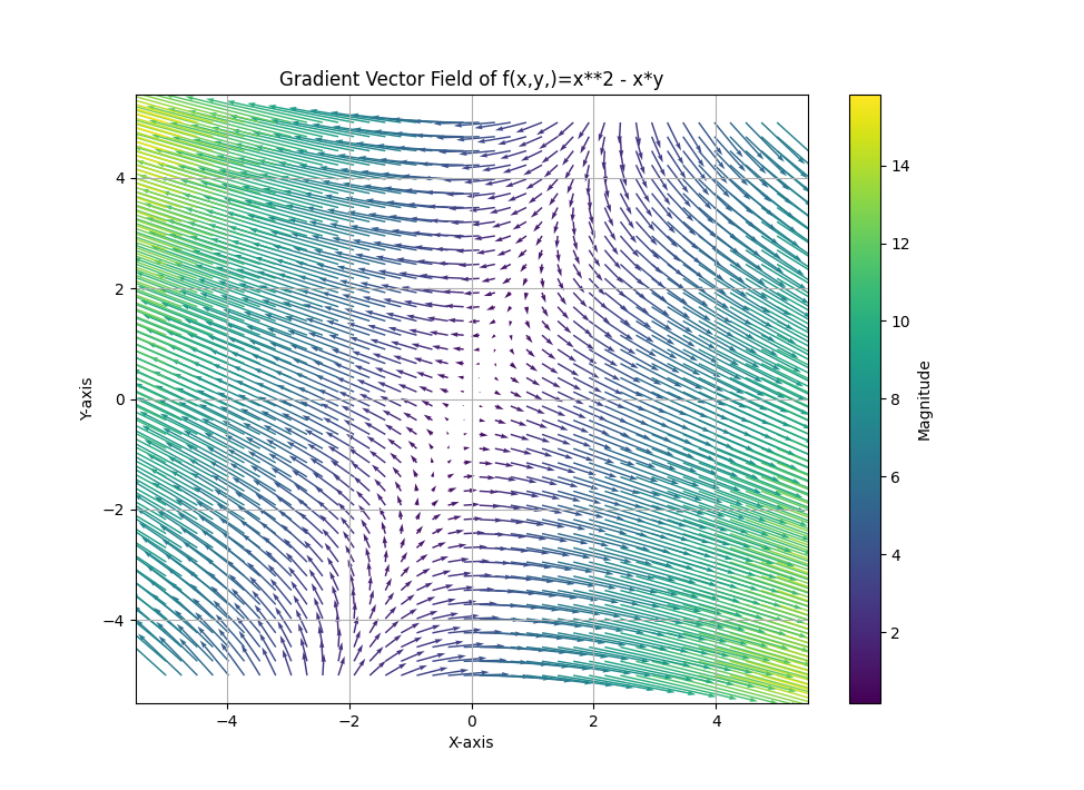
• 위 vector field는 \(f(x, y)\) 의 각 \((x, y)\) 에서의 gradient의 크기와 방향을 나타냅니다. 원점을 기준으로 우상향하는 대각선 방향에서의 graident의 크기가 매우 작은 것을 확인할 수 있습니다. 예시를 살펴보면 다음과 같습니다.

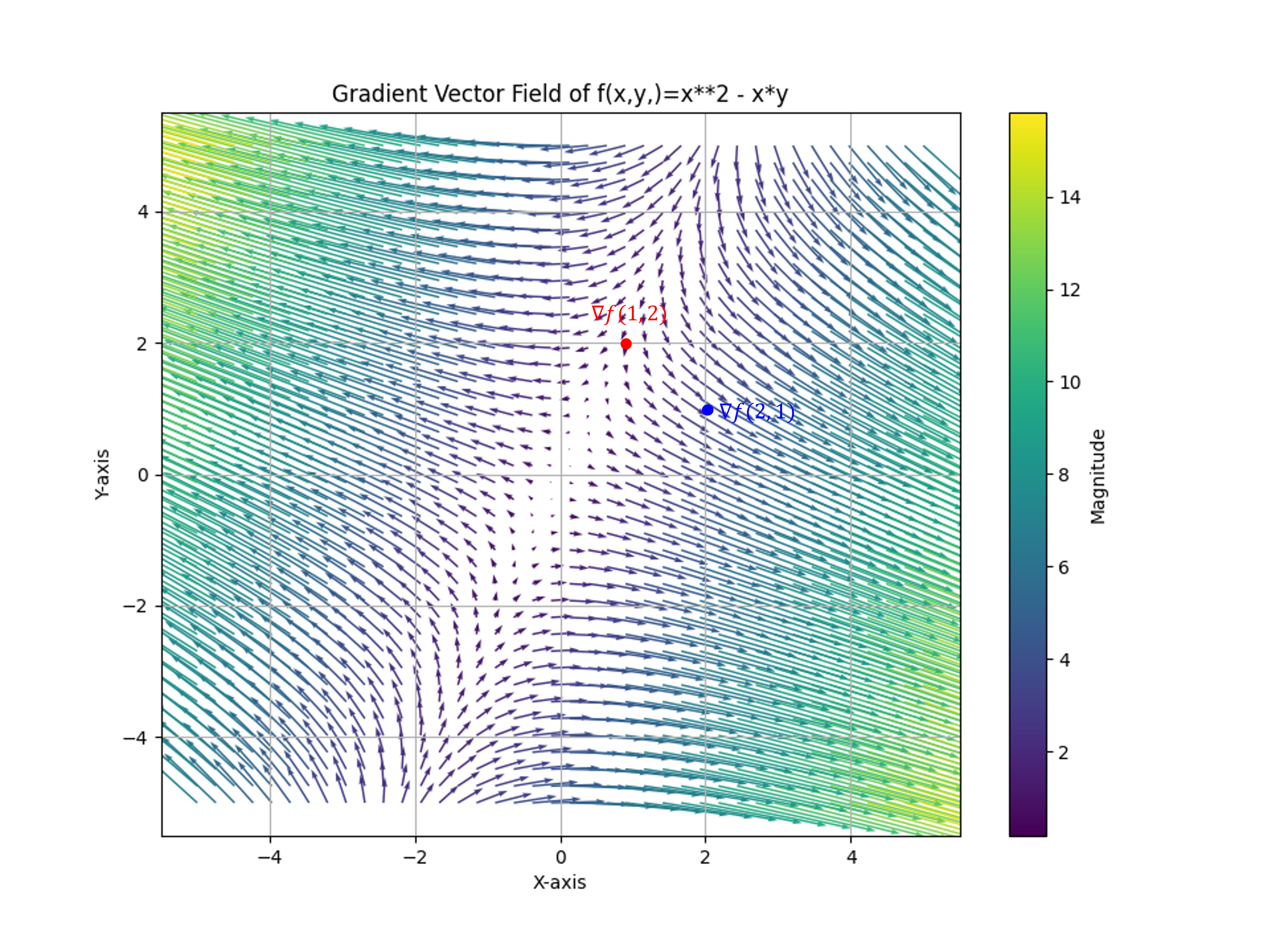
• \[\nabla f(1, 2) = \begin{bmatrix} 2(1) - 2 \\ -(1) \end{bmatrix} = \begin{bmatrix} 0 \\ -1 \end{bmatrix}\]
• \[\Vert \nabla f(1, 2) \Vert = \sqrt{0^{2} + (-1)^{2}} =1\]
• \[\nabla f(2, 1) = \begin{bmatrix} 2(2) - 1 \\ -(2) \end{bmatrix} = \begin{bmatrix} 3 \\ -2 \end{bmatrix}\]
• \[\Vert \nabla f(2, 1) \Vert = \sqrt{3^{2} + (-2)^{2}} = \sqrt{13}\]

• 이와 같은 방법으로 Graident를 구하면 각 위치에서의 Gradient를 이용하여 Vector Field를 생성할 수 있고 각 위치의 변화량 또한 확인할 수 있습니다.

• \[f(x, y, z) = x - xy + z^{2}\]
• \[\nabla f(x, y, z) = \begin{bmatrix} \frac{\partial}{\partial x} (x - xy + z^{2}) \\ \frac{\partial}{\partial y} (x - xy + z^{2}) \\ \frac{\partial}{\partial z} (x - xy + z^{2}) \end{bmatrix} = \begin{bmatrix} 1 - y \\ -x \\ 2z \end{bmatrix}\]

• 3개의 변수를 이용하여 gradient를 구해도 원리는 같습니다. 3개의 변수를 이용하여 vector field를 나타내면 아래와 같이 3차원 공간으로 나타나는 것을 볼 수 있습니다.

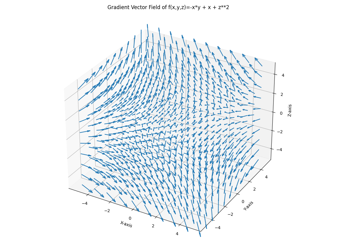
• gradient를 구한 결과 \(z\) 에 대한 변화량이 가장 큰 것을 알 수 있습니다. 따라서 위 vector field에서도 \(z\) 가 커지면 각 벡터의 크기도 가장 영향을 많이 받는 것을 확인할 수 있습니다.

• \[f(x, y) = -x^{4} + 4(x^{2} - y^{2}) - 3\]
• \[\nabla f(x, y) = \begin{bmatrix} \frac{\partial}{\partial x} (-x^{4} + 4(x^{2} - y^{2}) - 3 ) \\ \frac{\partial}{\partial y} (-x^{4} + 4(x^{2} - y^{2}) - 3) \end{bmatrix} = \begin{bmatrix} -4x^{3} + 8x \\ -8y \end{bmatrix}\]

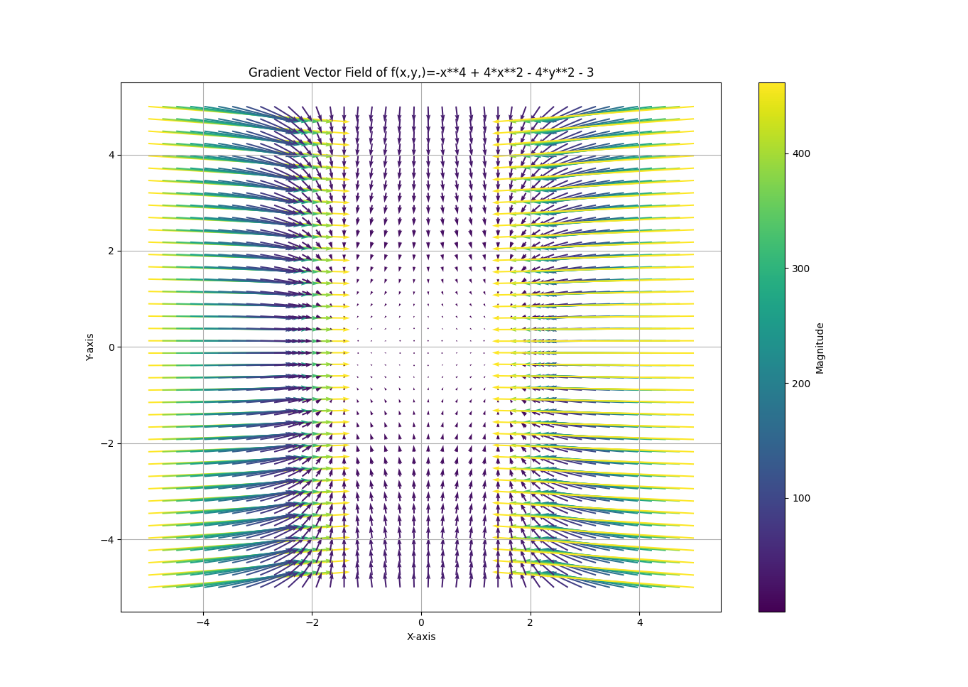
• 위 예제에서도 동일하게 Gradient를 적용하여 Vector Field를 시각화 하였습니다. 위 그림을 통하여 Gradient의 방향 및 크기를 통해 optimization 시 수렴할 수 있는 Local/Global Minimum 위치 등을 확인할 수 있습니다.

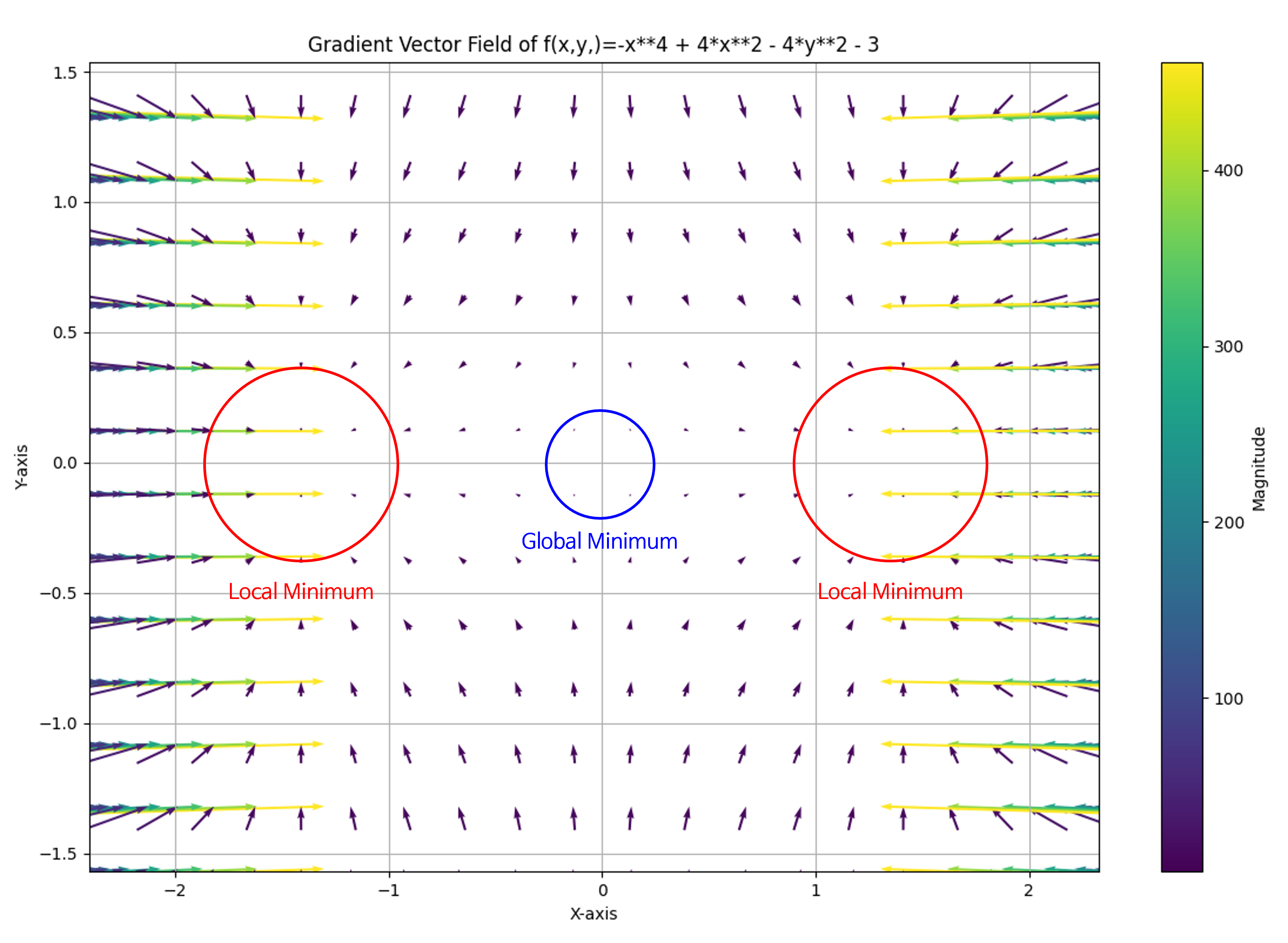
• 확대해서 살펴보면 위 그림과 같습니다.

Python을 이용한 Gradient 계산

• Python의 sympy를 이용하면 Gradient를 쉽게 구할 수 있습니다. sympy의 diff 함수를 이용하면 원하는 변수의 미분값을 쉽게 구할 수 있기 때문입니다.
• 앞에서 살펴본 예제를 실제 파이썬 코드를 통하여 어떻게 구하는 지 한번 살펴보도록 하겠습니다.

from sympy import symbols, diff, Matrix, latex

# Define the variables
variables = symbols('x y')
x, y = variables

# Define the function
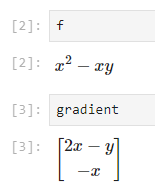
f = x**2 - x*y

# Calculate the gradient
gradient = Matrix([diff(f, var) for var in variables])
latex_code = latex(gradient)

# Output the gradient
print("Gradient of f:", gradient)
# Gradient of f: Matrix([[2*x - y], [-x]])
print("LaTex of gradient of f", latex_code)
# \left[\begin{matrix}2 x - y\\- x\end{matrix}\right]

• vector field를 구하는 코드는 다음과 같습니다.

import numpy as np
import matplotlib.pyplot as plt
from sympy import symbols, diff, lambdify

num_variable = 2

if num_variable == 2:
    # Step 1: Define the variables and function
    x, y = symbols('x y')
    f = -x**4 + 4*(x**2 - y**2) - 3
    # f = x**2 - x*y

    # Step 2: Compute the gradient symbolically
    gradient = [diff(f, var) for var in (x, y)]

    # Step 3: Create a numerical version of the gradient expressions
    grad_f = lambdify((x, y), gradient)

    # Step 4: Create a grid of points
    X, Y = np.meshgrid(np.linspace(-5, 5, 40), np.linspace(-5, 5, 40))

    # Step 5: Evaluate the gradient numerically at each point
    U, V = grad_f(X, Y)

    # Calculate the magnitude of the vectors
    magnitude = np.sqrt(U**2 + V**2)
    mean_magnitude = np.mean(magnitude)

    # # Step 6: Plot the vector field using quiver
    plt.figure(figsize=(8, 6))
    quiver  = plt.quiver(X, Y, U, V, magnitude, angles='xy', scale_units='xy', scale=mean_magnitude, cmap='viridis')

    # Adding a color bar to indicate the magnitude
    plt.colorbar(quiver, label='Magnitude')

    plt.xlabel('X-axis')
    plt.ylabel('Y-axis')
    plt.title('Gradient Vector Field of f(x,y,)={}'.format(str(f)))
    plt.grid(True)
    plt.show()
    
elif num_variable == 3:
    # # Define the variables and function
    x, y, z = symbols('x y z')
    f = x - x*y + z**2

    # # Compute the gradient symbolically
    gradient = [diff(f, var) for var in (x, y, z)]

    # # Create a numerical version of the gradient expressions
    grad_f = lambdify((x, y, z), gradient)

    # # Create a grid of points
    X, Y, Z = np.meshgrid(np.linspace(-5, 5, 10), np.linspace(-5, 5, 10), np.linspace(-5, 5, 10))

    # # Evaluate the gradient numerically at each point
    U, V, W = grad_f(X, Y, Z)

    # Calculate the magnitude of the vectors
    magnitude = np.sqrt(U**2 + V**2 + W**2)
    
    # Plot the vector field using quiver in 3D, colored by magnitude
    fig = plt.figure(figsize=(10, 8))
    ax = fig.add_subplot(111, projection='3d')
    quiver = ax.quiver(X, Y, Z, U, V, W, length=0.1, cmap='viridis')
    
    ax.set_xlabel('X-axis')
    ax.set_ylabel('Y-axis')
    ax.set_zlabel('Z-axis')
    ax.set_title('Gradient Vector Field of f(x,y,z)={}'.format(str(f)))
    plt.show()

Jacobian의 정의 및 예시

• 위키피디아의 Jacobian의 정의를 찾아보면 “The Jacobian matrix is the matrix of all first-order partial derivatives of a vector-valued function” 으로 나옵니다. 즉, Jacobian은 모든 벡터들의 1차 편미분값으로 구성된 행렬이고 각 행렬의 값은 vector-valued multivariable function일 때의 미분값으로 정의됩니다. 관련 용어 및 내용은 아래 내용을 천천히 읽어보시면 충분히 이해할 수 있도록 설명하였습니다.

• Jacobian은 다양한 문제에서 approximation 접근법을 사용할 때 자주 사용 되는 방법입니다.
• 예를 들어 비선형 칼만필터를 사용할 때, 비선형 식을 선형으로 근사시켜서 모델링 할 때 사용하는 Extended Kalman Filter가 대표적인 예가 될 수 있습니다. Jacobian은 정말 많이 쓰기 때문에 익혀두면 상당히 좋습니다.
• 먼저 Jacobian의 형태에 대하여 먼저 살펴보고 그 다음 Jacobian을 어떤 용도로 주로 사용하는 지 확인해 보도록 하겠습니다.

• 앞에서 Gradient는 다음과 같이 구하였었습니다.

• \[\nabla f(x, y, ...) = \begin{bmatrix} \frac{\partial f}{\partial x} \\ \frac{\partial f}{\partial y} \\ \vdots \end{bmatrix}\]

• 위 식에서 출력 형태는 vector입니다. Jacobian은 위 식의 출력 형태에서 부터 편미분을 시작합니다. 따라서 Jacobian은 vector-valued multivariable function을 편미분하는 것이라고 말할 수 있습니다.

• \[f(x, y, ...) = \begin{bmatrix} f_{1}(x, y, ...) \\ f_{2}(x, y, ...) \\ \vdots \end{bmatrix}\]

• 위 식에서 각 행의 함수에 대한 편미분의 결과는 Gradient 예제에서 살펴보았듯이 벡터가 됩니다. 따라서 vector-valued multivariable function \(f\) 의 Jacobian인 \(J_{f}\) 는 다음과 같은 행렬 결과를 가지게 됩니다.

• \[J_{f}(x, y, ...) = \begin{bmatrix} \frac{\partial f_{1}}{\partial x}(x, y, ...) & \frac{\partial f_{1}}{\partial y}(x, y, ...) & \cdots \\ \frac{\partial f_{2}}{\partial x}(x, y, ...) & \frac{\partial f_{2}}{\partial y}(x, y, ...) & \cdots \\ \vdots & \vdots & \ddots \end{bmatrix}\]

• 정리하면 Jacobian은 1개의 함수만을 이용하여 Gradient를 구하는 것에서 시작하여 N개 함수의 Gradient를 구하여 행렬로 만드는 것으로 이해할 수 있습니다. 이 때, 각 함수의 Gradient는 행벡터로 나열한 다음에 행방향으로 쌓아 행렬을 만듭니다.

• Jacobian은 다양한 용도로 사용될 수 있으나 가장 기본적으로 approximation을 할 때 주로 사용됩니다.

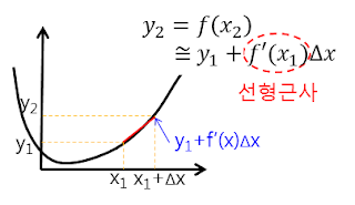
• 앞에서 말했듯이 Jacobian의 목적은 복잡하게 얽혀있는 식을 미분을 통하여 linear approximation 시킴으로써 간단한 근사 선형식을 만들어 주는 것입니다. 관련 내용은 테일러 급수와 연관되어 있으며 아래 내용에서 참조할 수 있습니다.
  • 참조 : https://gaussian37.github.io/math-mfml-taylor_series_and_linearisation/
  • 참조 : https://gaussian37.github.io/math-mfml-multivariate_calculus_and_jacobian/
• 위 그래프에서 미분 기울기를 통하여 \(\Delta x\) 후의 y값을 선형 근사하여 예측하는 것과 비슷한 원리 입니다.
• 그런데 위 그래프에서 알고 싶은 것은 \(f'(x_{1})\) 에서의 함수 입니다. 위 그래프에서 \(f'(x_{1})\) 이 기울기이기 때문에, \(f'(x_{1}) \times \Delta x \approx y_{2} - y_{1}\) 으로 근사화할 수 있기 때문입니다.

• 다시 한번 Jacobian을 행렬로 표현하면 다음과 같습니다.

• \[J = \frac{\partial y}{\partial x} = \frac{\partial f(x)}{\partial x} = \begin{bmatrix} \frac{\partial f_{1}}{\partial x_{1}} & \cdots & \frac{\partial f_{1}}{\partial x_{m}} \\ \vdots & \ddots & \vdots \\ \frac{\partial f_{n}}{\partial x_{1}} & \cdots & \frac{\partial f_{n}}{\partial x_{m}} \end{bmatrix}\]

• 여기서 J가 앞의 그래프 예시에 있는 함수 \(f'(x)\) 입니다. 따라서 다음과 같이 식을 정리할 수 있습니다.

• \[y_{i+1} = f(x_{i+1}) \approx y_{i} + \frac{\partial f(x_{i})}{\partial x_{i}} \Delta x = y_{i} + J \Delta x\]

• 또는 함수 \(f\) 에서 \(p\) 지점에서의 linear approximation을 나타내기 위해 다음과 같이 수식을 써서 표현하기도 합니다.

• \[f(x) \approx f(p) + J_{f}(p)(x - p)\]

Python을 이용한 Jacobian 계산

• Jacobian은 \(n \times m\) 크기의 행렬이며 \(n\) 개의 함수식과 \(m\) 개의 변수를 이용하여 다음과 같이 구해짐을 확인하였습니다. 편의상 변수는 \(x_{i}\) 로 나타내겠습니다.

• \[J = \begin{bmatrix} \frac{\partial f_{1}}{\partial x_{1}} & \frac{\partial f_{1}}{\partial x_{2}} & \cdots & \frac{\partial f_{1}}{\partial x_{m-1}} & \frac{\partial f_{1}}{\partial x_{m}} \\ \frac{\partial f_{2}}{\partial x_{1}} & \frac{\partial f_{2}}{\partial x_{2}} & \cdots & \frac{\partial f_{2}}{\partial x_{m-1}} & \frac{\partial f_{2}}{\partial x_{m}} \\ \vdots & \vdots & \ddots & \vdots & \vdots& \\ \frac{\partial f_{n-1}}{\partial x_{1}} & \frac{\partial f_{n-1}}{\partial x_{2}} & \cdots & \frac{\partial f_{n-1}}{\partial x_{m-1}} & \frac{\partial f_{n-1}}{\partial x_{m}} \\ \frac{\partial f_{n}}{\partial x_{1}} & \frac{\partial f_{n}}{\partial x_{2}} & \cdots & \frac{\partial f_{n}}{\partial x_{m-1}} & \frac{\partial f_{n}}{\partial x_{m}} \end{bmatrix}\]

• 위 식에서 Jacobian을 구하기 위한 편미분 계산은 파이썬의 sympy를 이용하면 간단하게 처리할 수 있습니다. (울프람 알파 등을 이용하여도 됩니다.)
• 이번 글에서는 Jacobian을 sympy를 이용하여 구하는 방법에 대하여 알아보도록 하겠습니다.

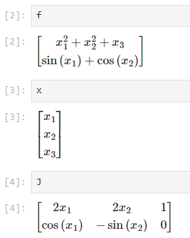
• 먼저 \(f_{i}\) 를 각각 정의해야 하고 편미분할 변수를 정의해야 합니다. 다루어볼 예제는 다음과 같습니다.

• \[F = \begin{bmatrix} x_{1}^{2} + x_{2}^{2} + x_{3} \\ \sin{(x_{1})} + \cos{(x_{2})} \end{bmatrix}\]
• \[X = \begin{bmatrix} x_{1} & x_{2} & x_{3} \end{bmatrix}^{T}\]

• Jacobian의 정의에 맞게 각 행렬의 성분을 편미분 하면 다음 결과를 얻을 수 있습니다.

• \[J = \begin{bmatrix} \frac{f_{1}}{x_{1}} & \frac{f_{1}}{x_{2}} & \frac{f_{1}}{x_{3}} \\ \frac{f_{2}}{x_{1}} & \frac{f_{2}}{x_{2}} & \frac{f_{2}}{x_{3}} \end{bmatrix} = \begin{bmatrix} 2x_{1} & 2x_{2} & 1 \\ \cos{(x_{1})} & -\sin{(x_{2})} & 0 \end{bmatrix}\]

• 위 연산을 다음과 같이 계산할 수 있습니다.

from sympy import symbols, Matrix, sin, cos, lambdify
import numpy as np

# Step 1: Define the symbolic variables
x1, x2, x3 = symbols('x1 x2 x3')

# Step 2: Define the function vector
f = Matrix([x1**2 + x2**2 + x3, sin(x1) + cos(x2)])

# Step 3: Define the variable vector
x = Matrix([x1, x2, x3])

# Step 4: Compute the Jacobian matrix
J = f.jacobian(x)

• 따라서 코드를 이용해서도 동일한 결과를 얻을 수 있음을 확인하였습니다.
• 다음으로 임의의 입력에 대하여 Jacobian 행렬 연산 방법을 확인해 보겠습니다. 연산은 numpy를 사용하도록 코드를 작성하였습니다.

# Step 5: Convert the Jacobian to a NumPy function
jacobian_func = lambdify([x1, x2, x3], J, modules='numpy')

def jacobian_func_np(x1, x2, x3):
    matrix = np.array([
        [2*x1,        2*x2,       1],
        [np.cos(x1), -np.sin(x2), 0]
    ])
    return matrix 

# Step 6: Example usage with NumPy
input_vector = np.array([1.0, 2.0, 3.0])
jacobian_result = jacobian_func(*input_vector)

print("Jacobian matrix with lambdify at", input_vector, "is:")
print(np.array(jacobian_result))
print()
# Jacobian matrix with lambdify at [1. 2. 3.] is:
# [[ 2.          4.          1.        ]
#  [ 0.54030231 -0.90929743  0.        ]]

print("Jacobian matrix with numpy at", input_vector, "is:")
jacobian_result = jacobian_func_np(*input_vector)
print(np.array(jacobian_result))
# Jacobian matrix with numpy at [1. 2. 3.] is:
# [[ 2.          4.          1.        ]
#  [ 0.54030231 -0.90929743  0.        ]]

• 위 코드의 2가지 결과 모두 동일함을 알 수 있습니다. 첫번째 jacobian_func는 lambdify라는 모듈을 이용하여 Jacobian 행렬을 별도 변환 없이 바로 사용한 경우입니다. 반면 jacobian_func_np는 직접 numpy 배열로 변환하여 사용한 것으로 jacobian_func를 확인하기 위한 용도로 별도 정의하였습니다.
• 따라서 실제 사용할 때에는 jacobian_func를 사용하여 jacobian을 구하고 계산된 결과만 numpy로 받아서 사용하는 것을 권장드립니다.

• 다음은 원의 방정식에 대한 Jacobian을 구하는 형태의 예제를 살펴보도록 하겠습니다.
• 원의 방정식 \((x - a)^{2} + (y - b)^{2} = r^{2}\) 에서 \(a, b, r\) 에 대한 편미분을 통해 Jacobian을 계산합니다.
• 첫번째 예제로 복수 개의 식을 나열하기 위하여 직접 \((x, y)\) 를 대입하여 \(n\) 개의 식을 만들어 Jacobian을 구하는 방법과 \((x, y)\) 또한 변수화 하여 대수적으로 Jacobian을 구하는 방식을 차례대로 확인해 보겠습니다.

• \[(x - a)^{2} + (y - b)^{2} = r^{2}\]
• \[(a, b) \text{: center coordinates of the circle}\]
• \[r \text{: radius}\]
• \[\text{Jacobian with respect to the circle parameters (a, b, r)}\]

• \[\text{residual function: } r_{i} = \sqrt{(x_{i} - a)^{2} + (y_{i} - b)^{2}} - r\]

from sympy import symbols, Matrix, sqrt, lambdify
import numpy as np

# Define symbolic variables for the circle parameters and points
a, b, r = symbols('a b r')

# Example data points
points = np.array([[1, 7], [5, 8], [9, 8]])

# Example circle parameters (a, b, r)
params = [5.0, 5.0, 3.0]

# Define the residual function for a single point
residuals = Matrix([])
for x, y in points:
    residuals = residuals.row_insert(residuals.shape[0], Matrix([sqrt((x - a)**2 + (y - b)**2) - r]))

# Compute the Jacobian matrix of the residual function
jacobian = residuals.jacobian([a, b, r])

# Convert the Jacobian to a numerical function using lambdify
jacobian_func = lambdify([a, b], jacobian, 'numpy')

# Print the Jacobian matrix
print("Jacobian matrix (3x3):")
jacobian_result = jacobian_func(0, 0)
print(jacobian_result)

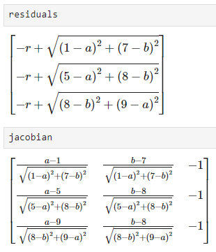
• 위 식에서 \(F\) 로 정의한 residuals와 \(J\) 인 jacobian을 구한 결과는 위 식과 같습니다.

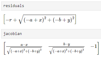
• 이번에는 약간 \((x, y)\) 또한 변수화 하여 Jacobian 행렬을 생성해 보도록 하겠습니다. 코드의 편의상 사용한 것이며 개념적으로 달라진 것은 없습니다.

from sympy import symbols, Matrix, sqrt, lambdify
import numpy as np

# Define symbolic variables for the circle parameters and points
a, b, r = symbols('a b r')
x, y = symbols('x y')

# Define the residual function for a single point
residuals = Matrix([sqrt((x - a)**2 + (y - b)**2) - r])

# Compute the Jacobian matrix of the residual function
jacobian = residuals.jacobian([a, b, r])

# Convert the Jacobian to a numerical function using lambdify
jacobian_func = lambdify([a, b, r, x, y], jacobian, 'numpy')

# Function to compute the Jacobian matrix for multiple points
def get_jacobian_results(params, points):
    a, b, r = params
    return np.array([jacobian_func(a, b, r, x, y) for x, y in points])

# Example data points
points = np.array([[1.0, 7.0], [4.0, 8.0], [9.0, 8.0]])

# Example circle parameters (a, b, r)
params = [5.0, 5.0, 3.0]

# Compute the 3x3 Jacobian matrix
jacobian_result = get_jacobian_results(params, points)

# Print the Jacobian matrix
jacobian_result_matrix = np.vstack(jacobian_result)
print("Jacobian matrix (3x3):")
print(jacobian_result_matrix)

Hessian의 정의 및 예시

• Hessian은 앞에서 간략히 정리한 바와 같이 scalar-valued function (1개의 함수)에 대하여 2차 편미분을 적용한 결과를 행렬로 나타낸 것을 의미하며 다음과 같이 정의됩니다.
• 먼저 2차 편미분은 다음과 같은 방식으로 표현합니다.

• \[\frac{\partial}{\partial \color{blue}{x}}\left( \frac{\partial f}{\partial \color{blue}{x}} \right) = \frac{\partial^{2} f}{\partial \color{blue}{x}^{2}}\]
• \[\frac{\partial}{\partial \color{blue}{x}}\left( \frac{\partial f}{\partial \color{red}{y}} \right) = \frac{\partial^{2} f}{\partial \color{blue}{x} \partial \color{red}{y}}\]
• \[\frac{\partial}{\partial \color{red}{y}}\left( \frac{\partial f}{\partial \color{blue}{x}} \right) = \frac{\partial^{2} f}{\partial \color{red}{y} \partial \color{blue}{x}}\]
• \[\frac{\partial}{\partial \color{red}{y}}\left( \frac{\partial f}{\partial \color{red}{y}} \right) = \frac{\partial^{2} f}{\partial \color{red}{y}^{2}}\]
• \[\text{Symmetry of second derivatives: } \frac{\partial^{2} f}{\partial \color{blue}{x} \partial \color{red}{y}} = \frac{\partial^{2} f}{\partial \color{red}{y} \partial \color{blue}{x}}\]

• \[H_{f} = \begin{bmatrix} \frac{\partial^{2} f}{\partial x^{2}} & \frac{\partial^{2} f}{\partial x \partial y} & \frac{\partial^{2} f}{\partial x \partial z} & \cdots \\ \frac{\partial^{2} f}{\partial y \partial x} & \frac{\partial^{2} f}{\partial y^{2}} & \frac{\partial^{2} f}{\partial y \partial z} & \cdots \\ \frac{\partial^{2} f}{\partial z \partial x} & \frac{\partial^{2} f}{\partial z \partial y} & \frac{\partial^{2} f}{\partial z^{2}} & \cdots \\ \vdots & \vdots & \vdots & \ddots \end{bmatrix}\]

• 위 Hessian은 scalar-valued function \(f\) 에 대하여 2차 편미분을 계산한 것을 확인할 수 있습니다. 또한 Hessian의 결과를 보면 Symmetry of second derivatives 성질로 인하여 Symmetric Matrix가 됨을 알 수 있습니다.
• 다음 예제를 살펴보도록 하겠습니다.

• \[\text{Hessian of } f(x, y) = x^{3} - 2xy - y^{6} \text{ at the point } (1, 2)\]

• \[f_{x}(x, y) = \frac{\partial}{\partial x}(x^{3} - 2xy - y^{6}) = 3x^{2} - 2y\]
• \[f_{y}(x, y) = \frac{\partial}{\partial y}(x^{3} - 2xy - y^{6}) = -2x -6y^{5}\]
• \[f_{xx}(x, y) = \frac{\partial}{\partial x}(3x^{2} - 2y) = 6x\]
• \[f_{xy}(x, y) = \frac{\partial}{\partial y}(3x^{2} - 2y) = -2\]
• \[f_{yx}(x, y) = \frac{\partial}{\partial x}(-2x -6y^{5}) = -2\]
• \[f_{yy}(x, y) = \frac{\partial}{\partial y}(-2x -6y^{5}) = -30y^{4}\]

• \[H_{f(x, y)} = \begin{bmatrix} f_{xx}(x, y) & f_{xy}(x, y) \\ f_{yx}(x, y) & f_{yy}(x, y) \end{bmatrix} = \begin{bmatrix} 6x & -2 \\ -2 & -30y^{4} \end{bmatrix}\]
• \[H_{f(1, 2)} = \begin{bmatrix} 6(1) & -2 \\ -2 & -30(2)^{4} \end{bmatrix}= \begin{bmatrix} 6 & -2 \\ -2 & -480 \end{bmatrix}\]

• Hessian은 각 성분이 2차 편미분의 결과를 저장하고 있습니다. 2차 편미분은 curvature (곡률, 변화율)을 의미합니다.
• 따라서 Hessian의 Eigenvalue와 Eigenvector는 curvature의 Principle Component가 됩니다.
• 만약 모든 Eigenvalue의 곱이 양수이면 Eigenvalue 각각이 모두 양수이거나 모두 음수인 경우가 됩니다. 즉, 곡률의 방향이 모두 같은 방향이 되어 convex한 형태를 가지게 되고 global optimization을 구할 수 있는 형태가 됩니다. 반면 모든 Eigenvalue의 곱이 음수이면 곡률의 방향이 다른 성분이 있으므로 saddle point 형태가 되어 global optimization을 구할 수 없습니다.
  • 링크 그림 참조 : https://gaussian37.github.io/math-mfml-multivariate_calculus_and_jacobian/#hessian-1
• 만약 global optimization이 있는 상태라면 Hessian 행렬의 가장 왼쪽 상단의 값 하나만 추가적으로 확인하면 됩니다. 만약 좌상단의 값이 양수라면 curvature가 양수이므로 아래로 볼록한 convexity 형태를 가지게 되어 global minimum을 가지고 반대로 좌상단의 값이 음수라면 위로 볼록한 concavity 형태를 가지므로 global maximum을 가지게 됩니다.
• 모든 eigenvalue의 곱은 determinant를 의미하기 때문에 determinant가 양수인 지 음수인 지를 통하여 global optimization 유무를 구할 수 있습니다.

• eigenvalue는 Positive/Negative (Semi) Definite Matrix와도 연관이 있습니다. 따라서 다음과 같이 정리할 수 있으며 앞에서 다룬 내용과 동일한 의미를 가집니다.
  • 참조 : https://gaussian37.github.io/math-la-positive_definite_matrix/

• \[H_{f} \text{: convex on set A if, and only if, its Hessian matrix is positive semidefinite at all points on the set. }\]
• \[H_{f} \text{: strictly convex on set A if, and only if, its Hessian matrix is positive definite at all points on the set. }\]
• \[H_{f} \text{: concave on set A if, and only if, its Hessian matrix is negative semi-definite at all points on the set. }\]
• \[H_{f} \text{: strictly concave on set A if, and only if, its Hessian matrix is negative definite at all points on the set. }\]

• Hessian이 사용되는 대표적인 케이스는 multivariable function의 Taylor Series에서 2차 도함수를 구하는 데 사용됩니다. 가장 기본적인 single variable function의 Taylor Series는 다음과 같이 전개됩니다. 다음은 점 \(a\) 에서의 근사화 방법입니다.

• \[T(x) = \sum_{n=0}^{\infty} \frac{f^{(n)}(a)}{n!}(x - a)^{n} = f(a) + f'(a)(x-a) + \frac{1}{2}f''(a)(x-a)^{2} + \frac{1}{6}f'''(a)(x-a)^{3} + \cdots\]

• 위 식을 multivariable function의 Taylor Series로 나타내면 다음과 같습니다.

• \[T(x) = f(a) + (x-a)^{T}\nabla f(a) + \frac{1}{2}(x - a)^{T} H_{f}(x-a) + \cdots\]

Python을 이용한 Hessian 계산

• Hessian 또한 앞에서 사용한 sympy를 이용하여 구할 수 있습니다. 아래 예제는 앞에서 사용한 예시를 이용하였습니다.

import sympy as sp

# Step 1: Define symbolic variables
x, y = sp.symbols('x y')

# Step 2: Define the function f(x, y)
f = x**3-2*x*y-y**6

# Step 3: Compute the gradient of f
grad_f = [sp.diff(f, var) for var in (x, y)]

# Step 4: Compute the Hessian matrix
hessian = sp.Matrix([[sp.diff(g, var) for var in (x, y)] for g in grad_f])
hessian_func = sp.lambdify((x, y), hessian, 'numpy')

# Evaluate the function with numpy arrays (or numbers)
result = hessian_func(1, 2)  # Evaluating at x=1, y=2, z=3

# Display the Hessian matrix
print("Hessian Matrix: \n")
sp.pprint(Hessian)
# ⎡6⋅x    -2  ⎤
# ⎢           ⎥
# ⎢          4⎥
# ⎣-2   -30⋅y ⎦
print("Result: \n", result)
# Result: 
#  [[   6   -2]
#  [  -2 -480]]

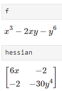
• 위 결과와 같이 원하는 Hessian 값을 코드를 통하여 구할 수 있습니다.

Calculus 관련 글 목차