포인트 클라우드 처리를 위한 open3d 사용법 정리

open3d로 point cloud 시각화 방법

아래 코드는 PointCloud 또는 Numpy 형태의 포인트 클라우드를 입력받아서 시각화 하는 기본적인 코드입니다.
추가적으로 좌표축도 같이 표현하고 있으며 R, G, B 색 순서로 X, Y, Z 축을 나타냅니다.

def show_open3d_pcd(pcd, show_origin=True, origin_size=3, show_grid=True):
    cloud = o3d.geometry.PointCloud()
    v3d = o3d.utility.Vector3dVector
    
    if isinstance(pcd, type(cloud)):
        pass
    elif isinstance(pcd, np.ndarray):
        cloud.points = v3d(pcd)
        
    coord = o3d.geometry.TriangleMesh().create_coordinate_frame(size=origin_size, origin=np.array([0.0, 0.0, 0.0]))
    
    # set front, lookat, up, zoom to change initial view
    o3d.visualization.draw_geometries([cloud, coord])

open3d로 grid 생성하는 방법

open3d로 포인트 클라우드를 읽었을 때, 그 포인트 클라우드의 대략적인 위치를 파악하기가 어렵습니다. 따라서 grid 형태로 거리를 참조할 수 있는 정보가 필요합니다.
아래 코드를 이용하면 XY, YZ, ZX 방향으로 grid를 그려서 포인트 클라우드의 위치를 파악하기 용이합니다.

import open3d as o3d
import numpy as np

import open3d as o3d
import numpy as np

def get_grid_lineset(h_min_val, h_max_val, w_min_val, w_max_val, ignore_axis, grid_length=1, nth_line=5):
    assert (h_min_val%2==0) and (h_max_val%2==0) and (w_min_val%2==0) and (w_max_val%2==0)
    
    num_h_grid = int(np.round((h_max_val - h_min_val) // grid_length, -1))
    num_w_grid = int(np.round((w_max_val - w_min_val) // grid_length, -1))
    
    num_h_grid_mid = num_h_grid // 2
    num_w_grid_mid = num_w_grid // 2
    
    grid_vertexes_order = np.zeros((num_h_grid, num_w_grid)).astype(np.int16)
    grid_vertexes = []
    vertex_order_index = 0
    
    for h in range(num_h_grid):
        for w in range(num_w_grid):
            grid_vertexes_order[h][w] = vertex_order_index
            if ignore_axis == 0:
                grid_vertexes.append([0, grid_length*w + w_min_val, grid_length*h + h_min_val])
            elif ignore_axis == 1:
                grid_vertexes.append([grid_length*h + h_min_val, 0, grid_length*w + w_min_val])
            elif ignore_axis == 2:
                grid_vertexes.append([grid_length*w + w_min_val, grid_length*h + h_min_val, 0])
            else:
                pass                
            vertex_order_index += 1       
            
    next_h = [0, 1]
    next_w = [1, 0]
    grid_lines = []
    grid_nth_lines = []
    for h in range(num_h_grid):
        for w in range(num_w_grid):
            here_h = h
            here_w = w
            for i in range(2):
                there_h = h + next_h[i]
                there_w = w +  next_w[i]   
                if (0 <= there_h and there_h < num_h_grid) and (0 <= there_w and there_w < num_w_grid):
                    if ((here_h % nth_line) == 0) and ((here_w % nth_line) == 0):
                        grid_nth_lines.append([grid_vertexes_order[here_h][here_w], grid_vertexes_order[there_h][there_w]])
                    elif ((here_h % nth_line) != 0) and ((here_w % nth_line) == 0) and i == 1:
                        grid_nth_lines.append([grid_vertexes_order[here_h][here_w], grid_vertexes_order[there_h][there_w]])
                    elif ((here_h % nth_line) == 0) and ((here_w % nth_line) != 0) and i == 0:
                        grid_nth_lines.append([grid_vertexes_order[here_h][here_w], grid_vertexes_order[there_h][there_w]])
                    else:
                        grid_lines.append([grid_vertexes_order[here_h][here_w], grid_vertexes_order[there_h][there_w]])

    color = (0.8, 0.8, 0.8)
    colors = [color for i in range(len(grid_lines))]
    line_set = o3d.geometry.LineSet(
        points=o3d.utility.Vector3dVector(grid_vertexes),
        lines=o3d.utility.Vector2iVector(grid_lines),
    )
    line_set.colors = o3d.utility.Vector3dVector(colors)
    
    color = (255, 0, 0)
    colors = [color for i in range(len(grid_nth_lines))]
    line_nth_set = o3d.geometry.LineSet(
        points=o3d.utility.Vector3dVector(grid_vertexes),
        lines=o3d.utility.Vector2iVector(grid_nth_lines),
    )
    line_nth_set.colors = o3d.utility.Vector3dVector(colors)
    
    return line_set, line_nth_set

def show_open3d_pcd(raw, show_origin=True, origin_size=3, 
                    show_grid=True, grid_len=1, 
                    voxel_size=0, 
                    range_min_xyz=(-80, -80, 0), range_max_xyz=(80, 80, 80)):
    '''
    - raw : numpy 2d array (size : (n, 3)) or o3d.geometry.PointCloud
    - show_origin : show origin XYZ coordinate. (X=red, Y=green, Z=Blue)
    - origin_size : size of origin coordinate.
    - show_grid : if true, show grid in xy, yz, zx plane with 'grid_len' length (default : gray line) and 5 times of 'grid_len' (default : red line)
    - voxel_size : voxel size to downsampling
    - range_min_xyz : grid min range of xyz orientation
    - range_max_xyz : grid max range of xyz orientation

    '''
    pcd = o3d.geometry.PointCloud()    
    
    if isinstance(raw, type(pcd)):
        pass
    elif isinstance(raw, np.ndarray):
        pcd.points = o3d.utility.Vector3dVector(raw)        
    if voxel_size > 0:
        pcd = pcd.voxel_down_sample(voxel_size=voxel_size)
        
    pcd_point = np.array(pcd.points)
    inrange_inds = (pcd_point[:, 0] > range_min_xyz[0]) & \
                    (pcd_point[:, 1] > range_min_xyz[1]) & \
                    (pcd_point[:, 2] > range_min_xyz[2]) & \
                    (pcd_point[:, 0] < range_max_xyz[0]) & \
                    (pcd_point[:, 1] < range_max_xyz[1]) & \
                    (pcd_point[:, 2] < range_max_xyz[2])    
    
    pcd_point = pcd_point[inrange_inds]
    filtered_raw = pcd_point
    pcd.points = o3d.utility.Vector3dVector(filtered_raw)
        
    x_min_val, y_min_val, z_min_val = range_min_xyz
    x_max_val, y_max_val, z_max_val = range_max_xyz
    
    coord = o3d.geometry.TriangleMesh().create_coordinate_frame(size=origin_size, origin=np.array([0.0, 0.0, 0.0]))
    
    ##################################### grid 생성 코드 ######################################
    lineset_yz, lineset_nth_yz = get_grid_lineset(z_min_val, z_max_val, y_min_val, y_max_val, 0, grid_len)
    lineset_zx, lineset_nth_zx = get_grid_lineset(x_min_val, x_max_val, z_min_val, z_max_val, 1, grid_len)
    lineset_xy, lineset_nth_xy = get_grid_lineset(y_min_val, y_max_val, x_min_val, x_max_val, 2, grid_len) 
    ###########################################################################################
    
    # set front, lookat, up, zoom to change initial view
    o3d.visualization.draw_geometries([pcd, coord,
                                       lineset_nth_yz, lineset_nth_zx, lineset_nth_xy,
                                       lineset_xy, lineset_yz, lineset_zx
                                      ])  

아래와 같이 호출하여 사용할 수 있습니다. 아래 bin 파일은 KITTI 데이터셋의 포인트 클라우드 데이터이며 bin 형태로 저장되어 있습니다. 아래 파일을 읽으면 열 방향으로 (X, Y, Z, Intensity) 순서로 읽을 수 있으며 (N, 4)의 크기 행렬을 가지게 됩니다.

raw = np.fromfile("00000001.bin", dtype=np.float32).reshape((-1, 4))
raw = raw[:, :3]
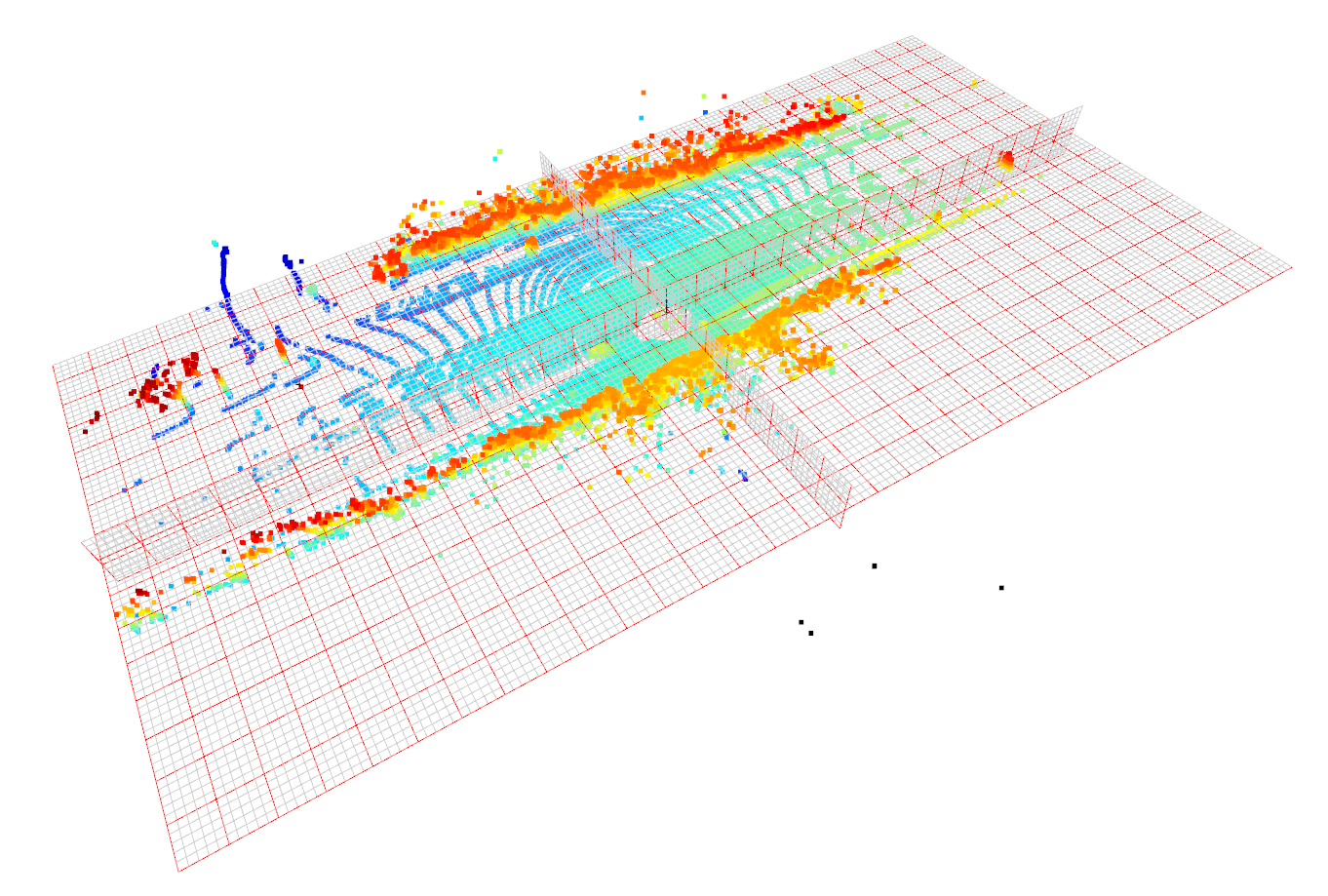
show_open3d_pcd(pcd, origin_size=3, range_min_xyz=(-40, -40, -5), range_max_xyz=(40, 40, 5))

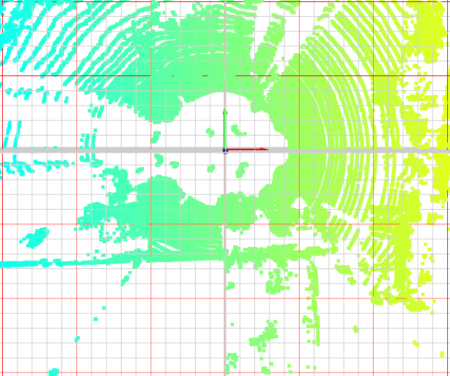
위 그림에서 연한 회색 선은 기본 값인 1m를 나타내고 빨간색 선은 기본 값의 5배인 5m를 나타냅니다. 위 코드에서 기본값을 2m로 바꾸면 빨간색 선은 5배인 10m를 나타냅니다.

show_open3d_pcd 함수에서 origin_size=3으로 지정하였고 origin이 3m 크기로 나타난 것을 확인할 수 있습니다.

range_min_xyz=(-40, -40, -5), range_max_xyz=(40, 40, 5) 의 옵션에 따라 x, y, z 방향으로 포인트들을 필터링하고 남겨진 포인트들을 적당한 마진을 추가하여 XYZ 평면에 표시한 형태입니다.

jupyter lab에서 open3d 시각화 방법

jupyter lab에서 open3d의 포인트를 시각화하는 방법을 정리하였습니다.
아래 코드에서 사용된 샘플 데이터인 000000.pcd는 KITTI 데이터 셋의 샘플 데이터이고 아래 링크에서 다운 받을 수 있습니다.
- 링크 : https://drive.google.com/file/d/1txU0Ou5VluSgqqBTJTC6G64s-pfDlccR/view?usp=sharing
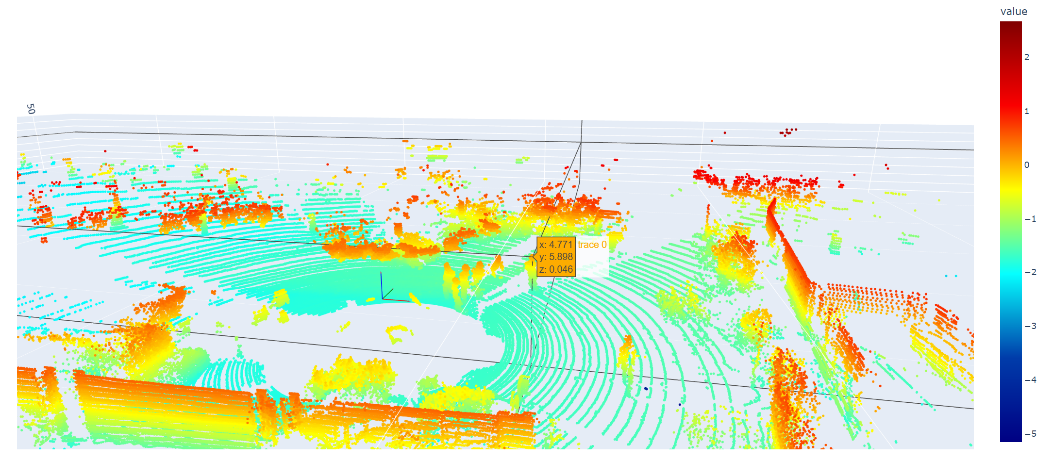
아래 코드를 이용하면 다음과 같이 시각화 할 수 있으며 장점은 다음과 같습니다.
- ① jupyter lab에서 ndarray 타입의 데이터를 바로 3D 환경에서 시각화 하여 볼 수 있습니다.
- ② 원하는 포인트의 좌표를 쉽게 확인할 수 있습니다.

def show_point_cloud(points, color_axis, width_size=1500, height_size=800, coordinate_frame=True):
    '''
    points : (N, 3) size of ndarray
    color_axis : 0, 1, 2
    '''
    assert points.shape[1] == 3
    assert color_axis==0 or color_axis==1 or color_axis==2   
    
    
    # Create a scatter3d Plotly plot
    plotly_fig = go.Figure(data=[go.Scatter3d(
        x=points[:, 0],
        y=points[:, 1],
        z=points[:, 2],
        mode='markers',
        marker=dict(
            size=1,
            color=points[:, color_axis], # Set color based on Z-values
            colorscale='jet', # Choose a color scale
            colorbar=dict(title='value') # Add a color bar with a title
        )
    )])

    x_range = points[:, 0].max()*0.9 - points[:, 0].min()*0.9
    y_range = points[:, 1].max()*0.9 - points[:, 1].min()*0.9
    z_range = points[:, 2].max()*0.9 - points[:, 2].min()*0.9

    # Adjust the Z-axis scale
    plotly_fig.update_layout(
        scene=dict(
            aspectmode='manual',
            aspectratio=dict(x=x_range, y=y_range, z=z_range), # Here you can set the scale of the Z-axis     
        ),
        width=width_size, # Width of the figure in pixels
        height=height_size, # Height of the figure in pixels
        showlegend=False
    )
    
    if coordinate_frame:
        # Length of the axes
        axis_length = 1

        # Create lines for the axes
        lines = [
            go.Scatter3d(x=[0, axis_length], y=[0, 0], z=[0, 0], mode='lines', line=dict(color='red')),
            go.Scatter3d(x=[0, 0], y=[0, axis_length], z=[0, 0], mode='lines', line=dict(color='green')),
            go.Scatter3d(x=[0, 0], y=[0, 0], z=[0, axis_length], mode='lines', line=dict(color='blue'))
        ]

        # Create cones (arrows) for the axes
        cones = [
            go.Cone(x=[axis_length], y=[0], z=[0], u=[axis_length], v=[0], w=[0], sizemode='absolute', sizeref=0.1, anchor='tail', showscale=False),
            go.Cone(x=[0], y=[axis_length], z=[0], u=[0], v=[axis_length], w=[0], sizemode='absolute', sizeref=0.1, anchor='tail', showscale=False),
            go.Cone(x=[0], y=[0], z=[axis_length], u=[0], v=[0], w=[axis_length], sizemode='absolute', sizeref=0.1, anchor='tail', showscale=False)
        ]

        # Add lines and cones to the figure
        for line in lines:
            plotly_fig.add_trace(line)
        for cone in cones:
            plotly_fig.add_trace(cone)

    # Show the plot
    plotly_fig.show()

# Extract the points as a NumPy array
pcd_path = "./000000.pcd"
pcd = o3d.io.read_point_cloud(pcd_path)
points = np.asarray(pcd.points)
show_point_cloud(points, 2)

실시간 데이터 시각화

다음 코드는 3D 포인트 데이터를 실시간으로 입력 받은 다음 실시간으로 데이터를 보여주어야 할 때 사용할 수 있습니다. 다음 코드에서는 실시간 데이터를 가정하기 위하여 임의의 랜덤 데이터를 입력으로 계속 받는 코드를 사용하였습니다.
grid를 그리는 코드는 앞에서 정의한 grid를 그리는 코드를 그대로 이용하였습니다.
아래 코드를 사용할 때에는 get_data() 함수 부분을 실제 데이터를 읽어오는 부분으로 교체하고 dt의 값을 변경하여 데이터를 읽어오는 주기를 조절해 줍니다. t_total 값은 얼마나 오래 코드를 실행할 지와 연관되어 있습니다.
중간에 코드를 멈추고 싶으면 Q를 눌러서 코드를 종료할 수 있도록 Callback 함수를 추가하였습니다.

import open3d as o3d
import numpy as np
import time
import glob

# random data
def get_data(): 
    normalized_points = np.random.rand(1000, 3) * 2 - 1.0 # range : -1 ~ 1
    normalized_points[:, 0] = normalized_points[:, 0] * 50
    normalized_points[:, 1] = normalized_points[:, 1] * 30
    normalized_points[:, 2] = normalized_points[:, 2] * 5
    return normalized_points

def quit_callback(vis):
    global exit_flag
    vis.close()
    exit_flag = True

# Global settings.
dt = 50/1000 # to add new points each dt secs.
t_total = 100 # total time to run this script.
exit_flag = False

# create visualizer and window.
vis = o3d.visualization.VisualizerWithKeyCallback()
vis.create_window()
vis.register_key_callback(ord('Q'), quit_callback)

# initialize pointcloud instance.
pcd = o3d.geometry.PointCloud()
points = np.array([
    [x_range[0], y_range[0], z_range[0]],
    [x_range[0], y_range[0], z_range[1]],
    [x_range[0], y_range[1], z_range[0]],
    [x_range[0], y_range[1], z_range[1]],
    [x_range[1], y_range[0], z_range[0]],
    [x_range[1], y_range[0], z_range[1]],
    [x_range[1], y_range[1], z_range[0]],
    [x_range[1], y_range[1], z_range[1]],
])

pcd.points = o3d.utility.Vector3dVector(points)
coord = o3d.geometry.TriangleMesh().create_coordinate_frame(size=3, origin=np.array([0.0, 0.0, 0.0]))
vis.add_geometry(pcd)
vis.add_geometry(coord)
vis.add_geometry(lineset_yz)
vis.add_geometry(lineset_zx)
vis.add_geometry(lineset_xy)
vis.add_geometry(lineset_nth_yz)
vis.add_geometry(lineset_nth_zx)
vis.add_geometry(lineset_nth_xy)

exec_times = []
current_t = time.time()
t0 = current_t

while current_t - t0 < t_total:
    previous_t = time.time()
    while current_t - previous_t < dt:                
        current_t = time.time()

    vis.poll_events()
    vis.update_renderer()
    pcd.points = o3d.utility.Vector3dVector()
    pcd.points.extend(get_data())
    vis.update_geometry(pcd)
    if exit_flag == True:
        break

vis.destroy_window()

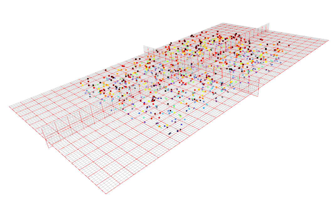
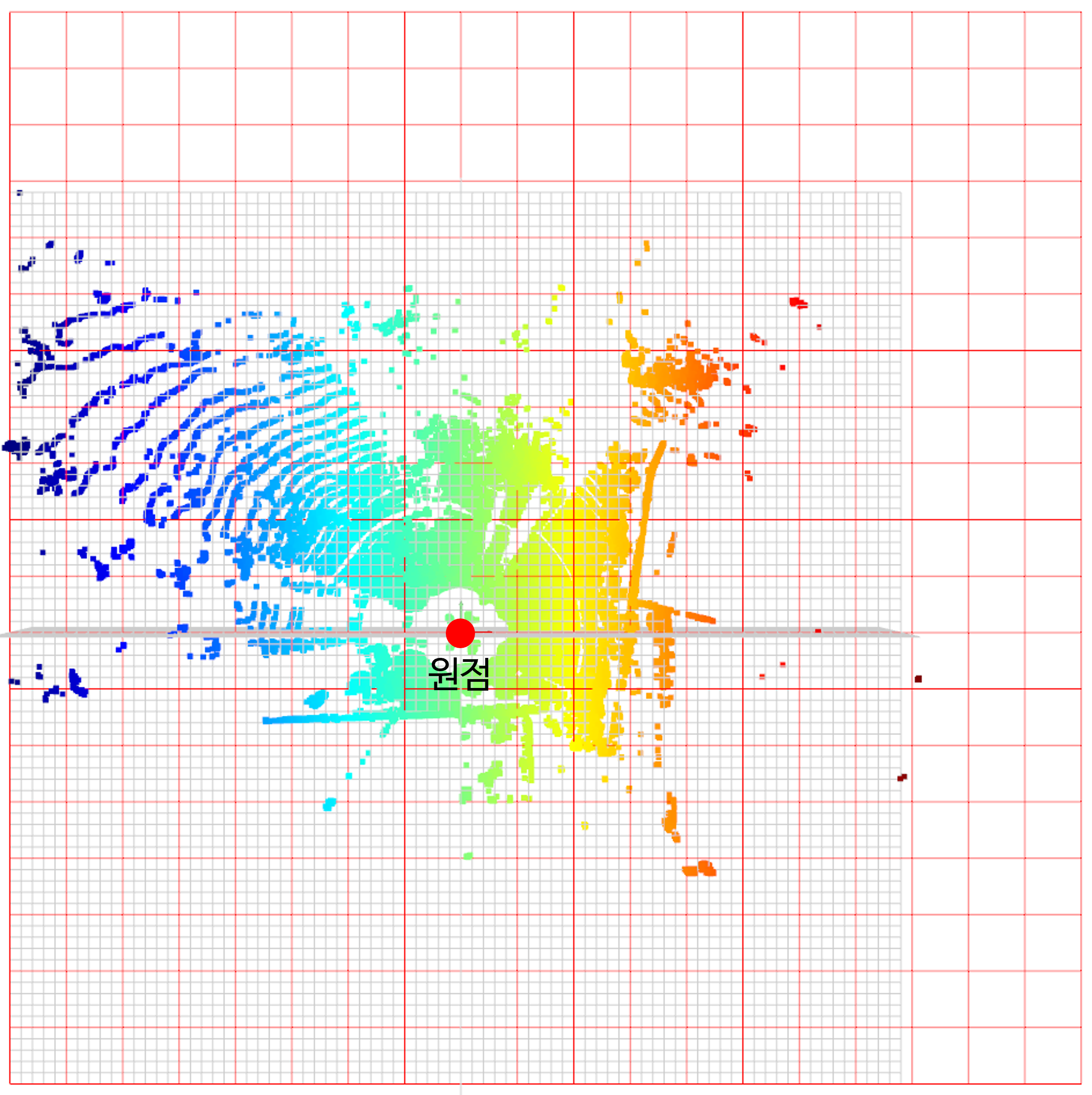
아래는 실시간으로 데이터를 읽어왔을 때, 순간 순간의 데이터가 어떻게 표현되는 지 나타낸 결과입니다.

연속된 point cloud 파일 읽어서 시각화

아래 방법은 연속된 포인트 클라우드를 이어서 보는 방법입니다. 아래 코드의 point_clouds와 같이 전체 포인트 클라우드를 등록하고 index를 변경해 가면서 시각화하는 컨셉입니다. index 변경은 N (Next), P(Previous)를 눌러서 앞 또는 뒤의 index 데이터를 불러오게 됩니다. Q를 입력하면 코드는 종료됩니다.
grid를 그리는 코드는 앞에서 정의한 grid를 그리는 코드를 그대로 이용하였습니다.

import open3d as o3d
import numpy as np
import time
import os
import glob

def get_local_pcd(path):
    # List of file paths for the .pcd files
    file_paths = glob.glob(path + os.sep + "*.pcd")
    file_paths.sort()
    
    # Read the point clouds and store them
    point_clouds = [np.array(o3d.io.read_point_cloud(file_path).points) for file_path in file_paths]
    return point_clouds
def load_point_cloud(file_path):
    return o3d.io.read_point_cloud(file_path)

# Initialize visualizer with key callbacks
vis = o3d.visualization.VisualizerWithKeyCallback()
vis.create_window()

# Load point clouds
point_clouds = get_local_pcd("./")

current_index = 0
pcd = o3d.geometry.PointCloud()
pcd.points = o3d.utility.Vector3dVector(point_clouds[current_index])

coord = o3d.geometry.TriangleMesh().create_coordinate_frame(size=3, origin=np.array([0.0, 0.0, 0.0]))

vis.add_geometry(pcd)
vis.add_geometry(coord)
vis.add_geometry(lineset_yz)
vis.add_geometry(lineset_zx)
vis.add_geometry(lineset_xy)
vis.add_geometry(lineset_nth_yz)
vis.add_geometry(lineset_nth_zx)
vis.add_geometry(lineset_nth_xy)

# Get view control and capture initial viewpoint
view_ctl = vis.get_view_control()
viewpoint_params = view_ctl.convert_to_pinhole_camera_parameters()

def update_visualization(vis, index, view_ctl, viewpoint_params):
    global pcd
    pcd.points = o3d.utility.Vector3dVector()
    pcd.points.extend(point_clouds[index])
    vis.update_geometry(pcd)

    view_ctl.convert_from_pinhole_camera_parameters(viewpoint_params)

def next_callback(vis):
    global current_index, viewpoint_params
    if current_index < len(point_clouds) - 1:
        # Capture current viewpoint before moving to next
        viewpoint_params = view_ctl.convert_to_pinhole_camera_parameters()
        current_index += 1
        update_visualization(vis, current_index, view_ctl, viewpoint_params)

def previous_callback(vis):
    global current_index, viewpoint_params
    if current_index > 0:
        # Capture current viewpoint before moving to next
        viewpoint_params = view_ctl.convert_to_pinhole_camera_parameters()
        current_index -= 1
        update_visualization(vis, current_index, view_ctl, viewpoint_params)

def quit_callback(vis):
    vis.close()  # Close the visualizer

# Register key callbacks
vis.register_key_callback(ord('N'), next_callback)
vis.register_key_callback(ord('P'), previous_callback)
vis.register_key_callback(ord('Q'), quit_callback)

# Run the visualizer
vis.run()
vis.destroy_window()

open3d에서 점 선택하는 방법

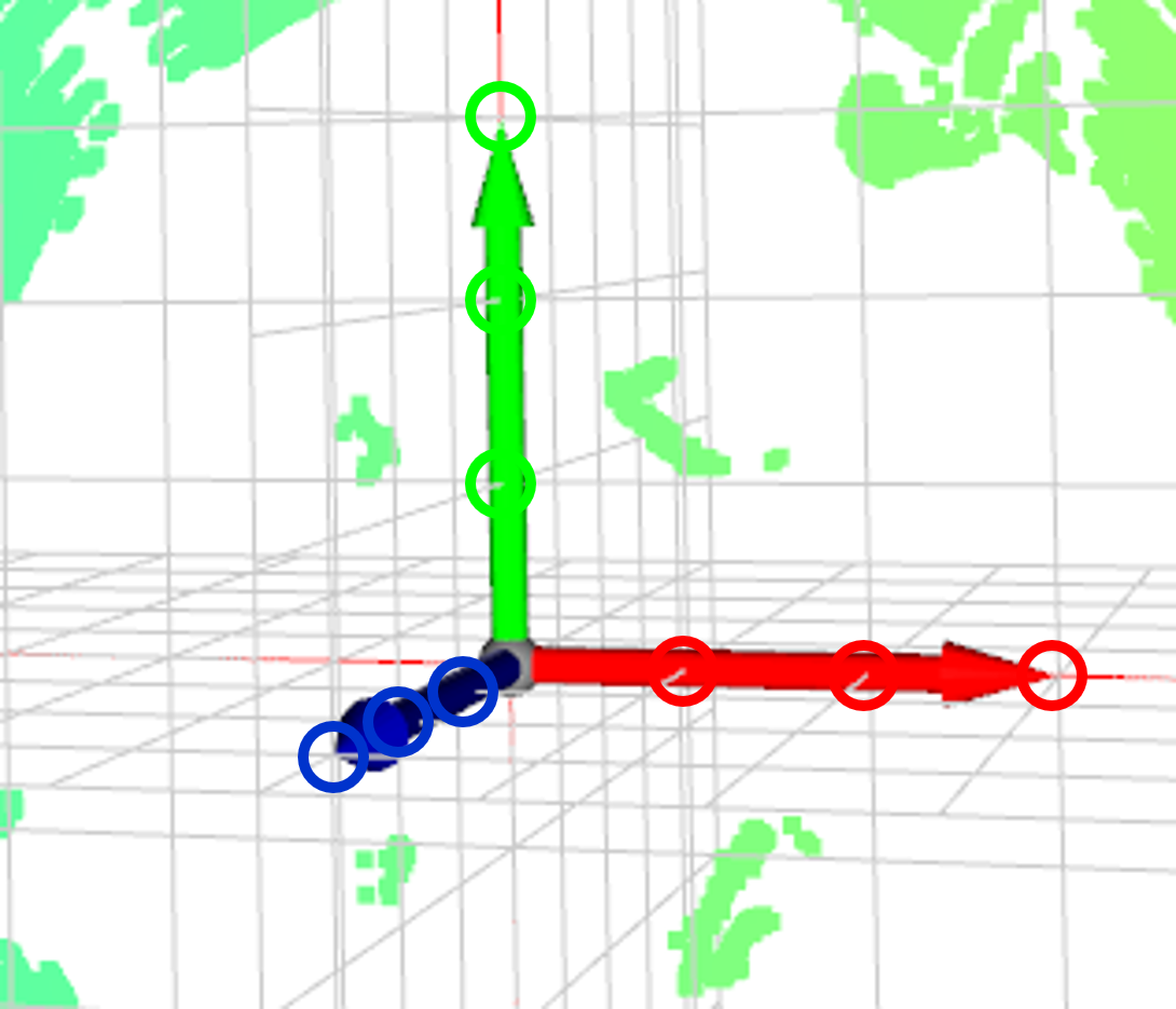
아래 코드의 vis.get_picked_points()를 이용하면 선택된 점을 구 형태로 표시를 해줍니다.
구를 선택할 때에는 shift + left mouse click으로 선택하면 되고 선택된 구를 해제할 때에는 shift + right mouse click으로 해제할 수 있습니다. 선택된 구의 크기는 shift +/-를 통하여 크기를 조절할 수 있습니다.
구를 선택하였을 때, 터미널에 선택된 구의 좌표가 임시적으로 출력됩니다.
모든 점들을 선택한 다음 창을 끄면 선택된 구의 정보를 확인할 수 있습니다.

import glob
import open3d as o3d
import numpy as np

file_paths = glob.glob("./*.pcd")
file_paths.sort()
point_clouds = [o3d.io.read_point_cloud(file_path) for file_path in file_paths]

pcd = point_clouds[0]
for i, pcd in enumerate(point_clouds):
    vis = o3d.visualization.VisualizerWithEditing()
    vis.create_window()
    vis.add_geometry(pcd)
    vis.run()  # user picks points
    vis.destroy_window()
    indices = vis.get_picked_points()
    pcd_points = np.array(pcd.points)

    print("\n{}th point cloud".format(i))
    for index in indices:
        print(index, pcd_points[index])

목차

open3d로 point cloud 시각화 방법

open3d로 grid 생성하는 방법

jupyter lab에서 open3d 시각화 방법

실시간 데이터 시각화

연속된 point cloud 파일 읽어서 시각화

open3d에서 점 선택하는 방법

open3d로 point cloud 시각화 방법

open3d로 grid 생성하는 방법

jupyter lab에서 open3d 시각화 방법

실시간 데이터 시각화

연속된 point cloud 파일 읽어서 시각화

open3d에서 점 선택하는 방법