Vehicle Dynamics와 Bicycle Model

Optimal State Estimation 글 목차

이번 글은 Andreas Geiger의 Self-Driving Cars 강의 내용을 참조하여 작성하였습니다.

Vehicle Dynamics

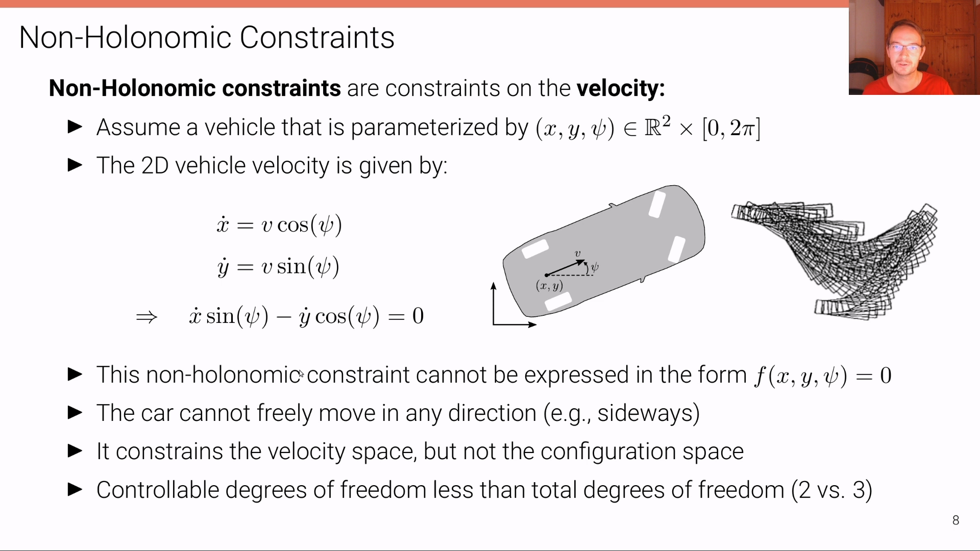
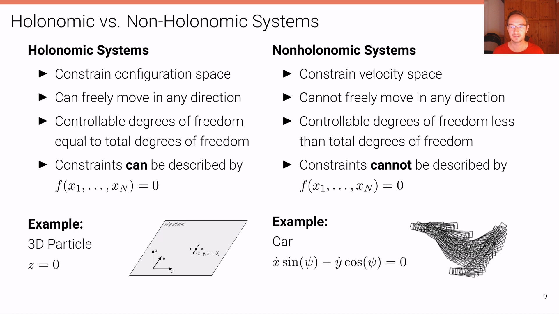
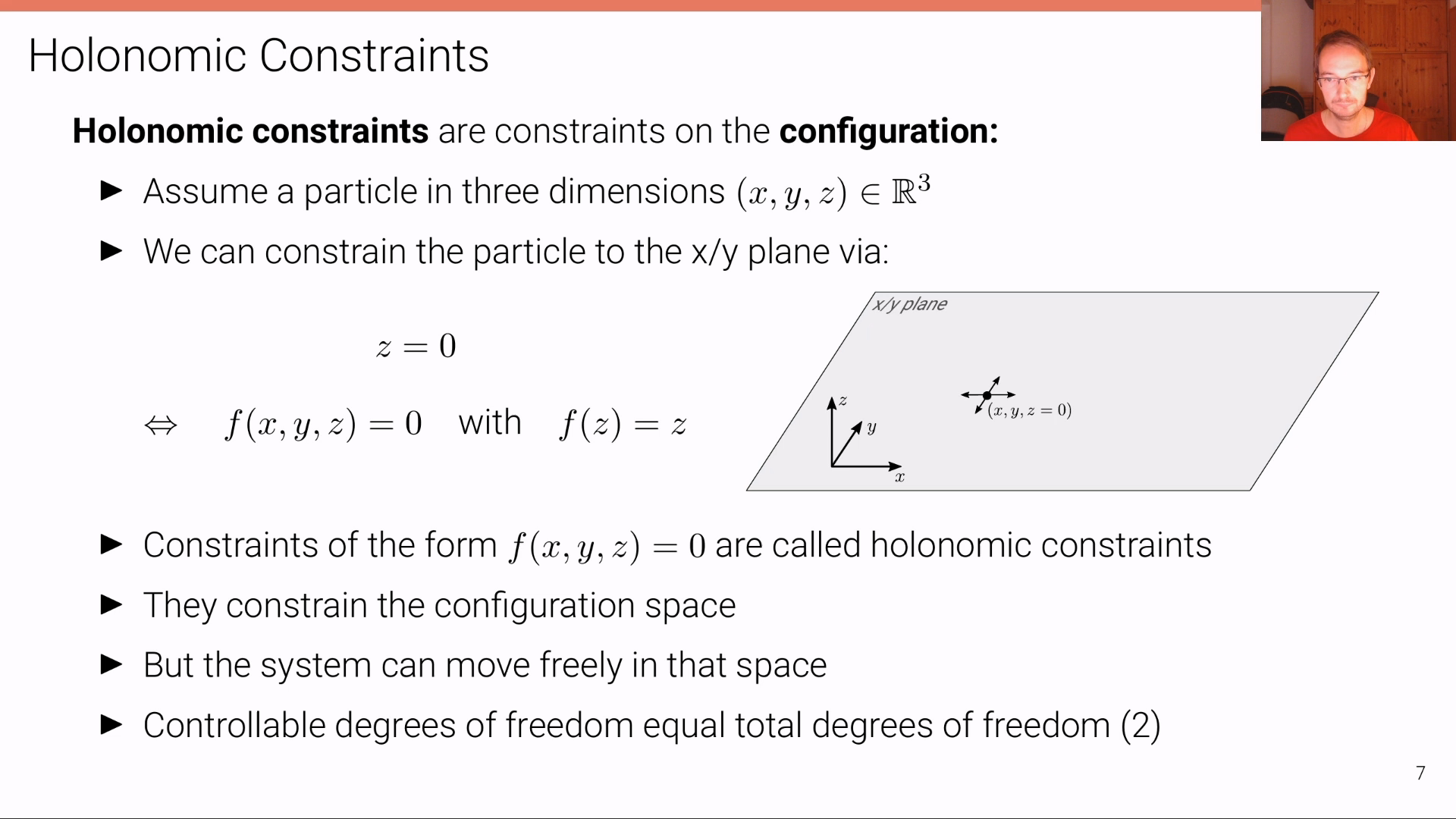
먼저 7, 8 슬라이드에서 설명하는 holonomic과 non-holonomic의 정의를 쉽게 설명한 글을 아래 링크를 통해 참조할 수 있습니다.
- 링크 : holonomic과 non-holonomic의 정의 설명

Kinematic Bicycle Model

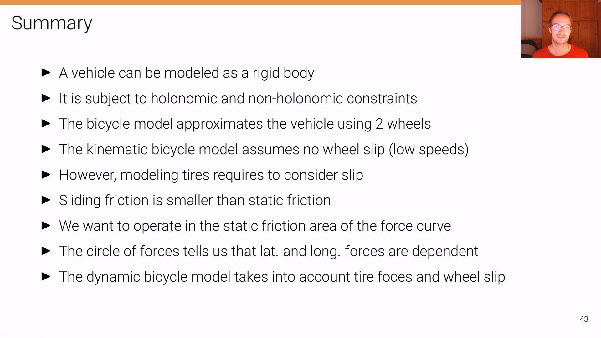
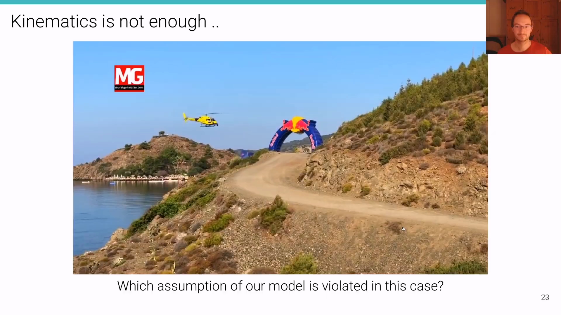
지금부터 Kinematic Bicycle Model에 대하여 살펴보도록 하겠습니다. 이 모델은 vehicle dynamics를 설명하는 모델 중 가장 간단한 모델이며 모델을 단순화하기 위하여 몇가지 가정을 전제로 모델링 됩니다.
먼저 이 모델은 바퀴가 미끄러짐이 없는 상황 (no wheel slip)을 전제로 합니다. 이 전제 조건은 저속 상황에서만 만족할 수 있으므로 주차 동작과 같은 제한된 저속 상태에서만 적용할 수 있습니다.
바퀴가 미끄러지는 현상은 아래 영상에서 확인할 수 있습니다.

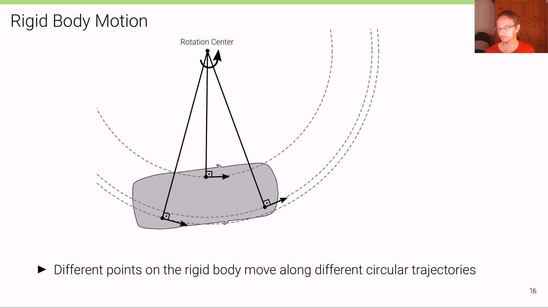
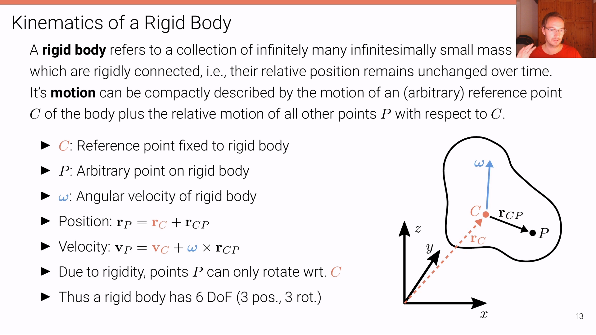
Kinematic Bicycle Model에서 다루는 차량은 Rigid Body Motion임을 전제로 합니다. 즉 차량의 각 부분들은 위치 변화가 없는 강체(Rigid Body)이며 회전 시에는 Rotation Center를 기준으로 회전을 하게 됩니다.
위 그림과 같이 차량의 다른 부분은 같은 Rotation Center를 가지지만 다른 반경을 두고 회전을 하게 되는 것을 알 수 있습니다.
위 그림에서 회전하는 방향에서의 속도를 회전 반경과 직교하는 방향으로 표현하였는데 이 부분은 앞으로 계산식에 사용됩니다.

Kinematic Bicycle Model에서는 차량이 4개의 바퀴를 가지고 있더라도 2개의 바퀴를 가지고 있는 것으로 근사화 하여 사용합니다. 따라서 위 그림과 같이 2개의 가상의 바퀴를 그려서 모델링하게 되며 이와 같은 이유로 Bicycle Model이라는 용어를 사용하게 됩니다.

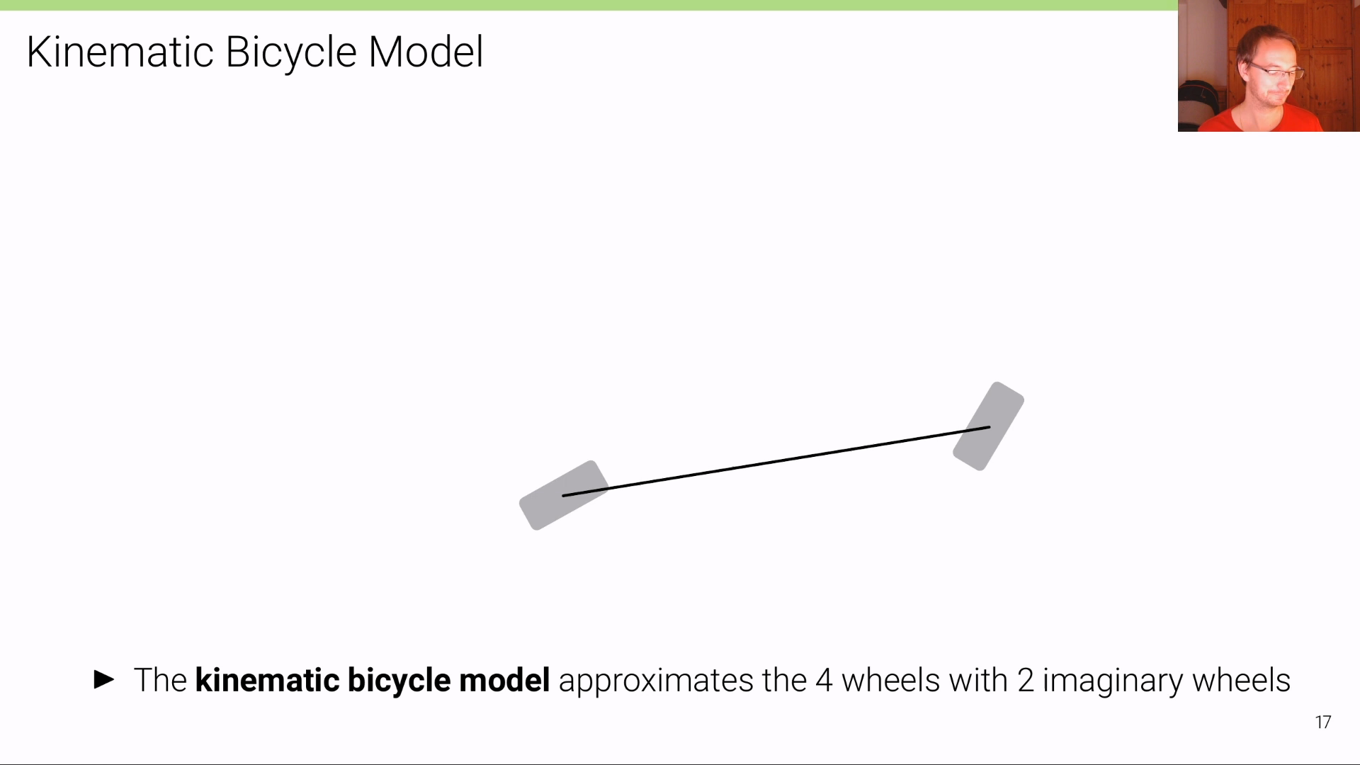
따라서 앞으로 사용할 차량의 형상은 자전거와 같이 2개의 바퀴를 가지며 2개의 바퀴는 하나의 축으로 전륜과 후륜이 연결된 형태로 사용됩니다.

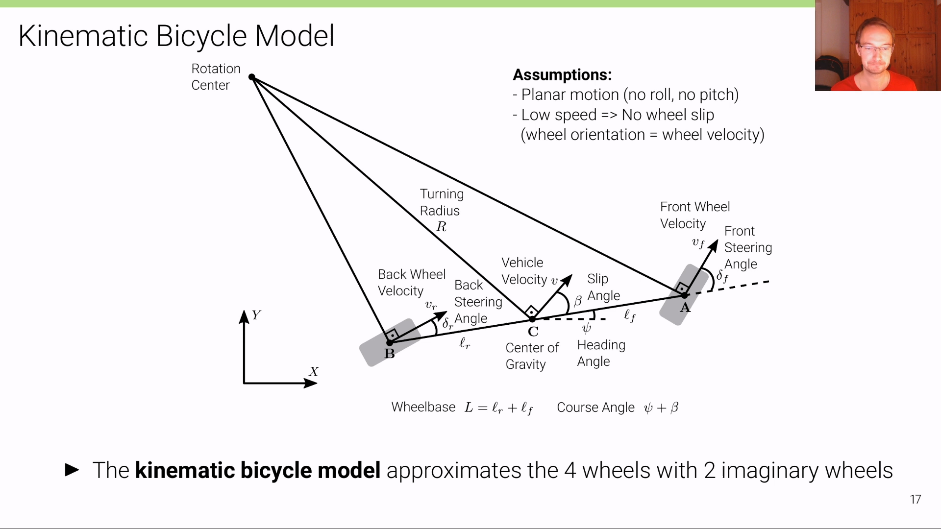
이와 같은 상태에서 Kinematic Bicycle Model은 몇가지 가정을 더 사용합니다.
먼저 2D Planar motion만을 가정하므로 3차원 회전 중 roll과 pitch가 없다고 가정합니다. 즉, \(Z\) 축 기준의 회전이 적용되는 2D Planar motion만 가정하므로 yaw 값만 존재합니다. 위 그림에서 \(\psi\) 로 표현된 방향 각도가 차량이 바라보는 방향 각도에 해당하며 이 값이 yaw가 됩니다.
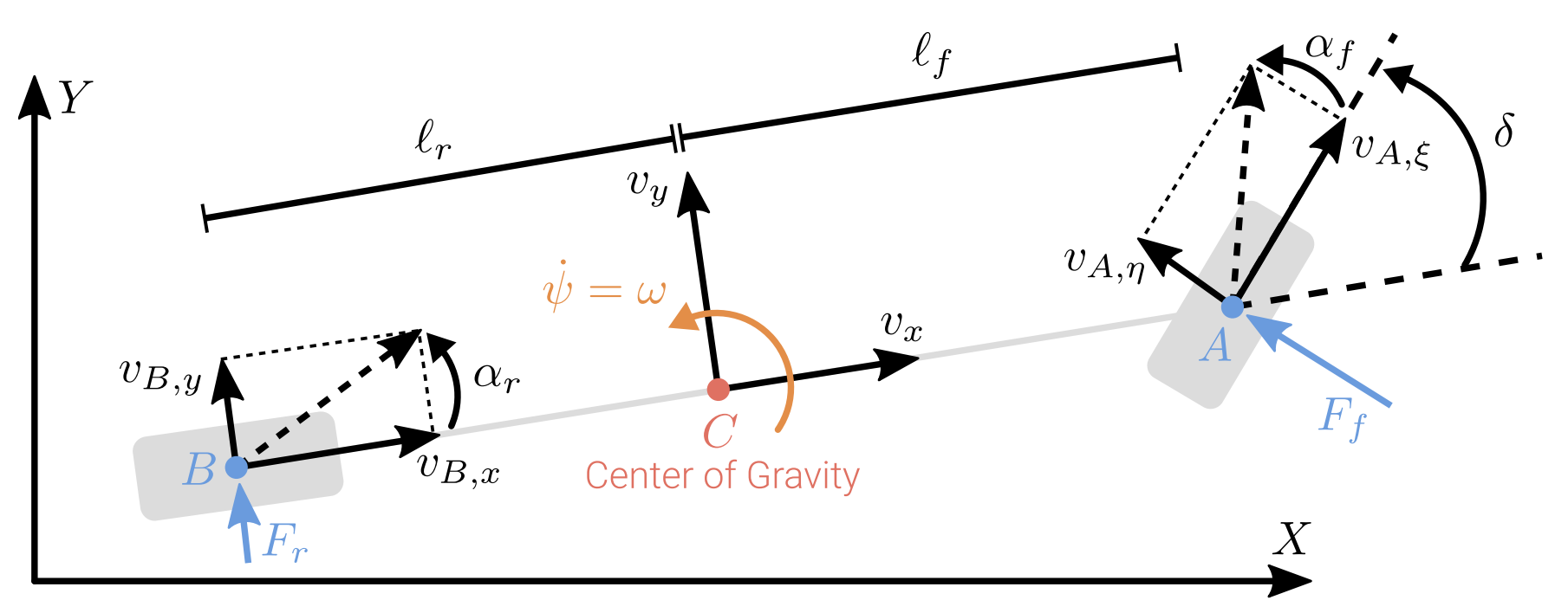
앞에서 설명하였듯이 Kinematic Bicycle Model에서는 바퀴 미끄러짐은 고려하지 않으며 바퀴의 속도에서는 방향 성분은 바퀴의 방향을 따릅니다.
위 그림에서 속도는 크게 3가지 종류가 있습니다. \(v_{f}, v_{r}\) 각각은 전륜 속도와 후륜 속도를 의미합니다. 차량에서는 실제 동력이 발생하는 위치가 차량의 앞쪽일 수 있고 또는 뒷쪽일 수 있기 때문에 전륜과 후륜의 속도가 다를 수 있습니다. 그리고 실제 차량의 속도를 \(v\) 라고 표현합니다.
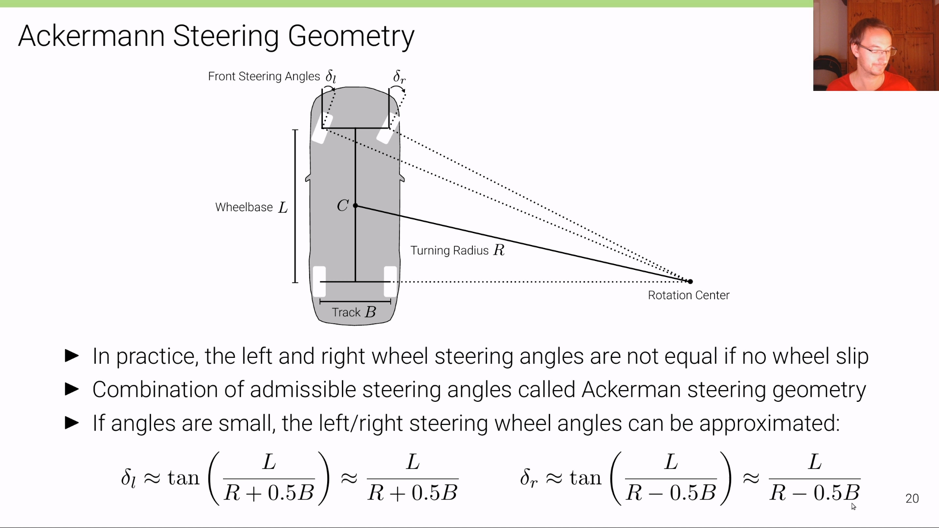
전륜과 후륜의 회전 상태 또한 다를 수 있기 때문에 위 그림과 같이 \(\delta_{f} , \delta_{r}\) 이 각각 정의되어 있습니다.
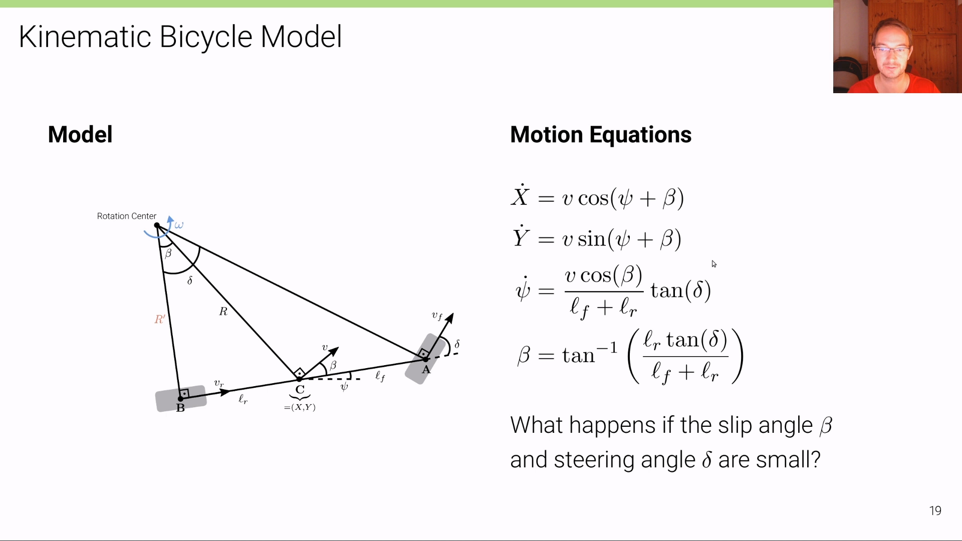
Kinematic Bicycle Model에서 고려해야 할 상황은 Slip Angle \(\beta\) 입니다. 위 그림과 같이 바퀴가 실제 향하는 방향이 있다고 하더라도 차량은 그 바퀴 방향대로 바로 움직이지 못합니다. 바퀴가 움직이는 방향과 차량의 위치를 대표하는 무게 중심 (Center of Gravity)의 위치가 다르고 관성으로 인하여 기존 진행 방향으로 미끄러지기 때문입니다. 따라서 차량은 Heading Angle \(\psi\) 방향으로 향하고 있으며 실제 움직이는 각도인 Course Angle은 \(\psi + \beta\) 가 됩니다. Kinematic Bicycle Model에서는 바퀴의 슬립은 고려하지 않지만 차량의 슬립은 차량 위치에 반영해야 하므로 존재한다고 보시면 됩니다.
마지막으로 Turning Radius \(R\) 은 차량이 Rotation Center로 부터 원을 그리며 회전한다고 할 때의 반지름 \(R\) 을 의미합니다. 회전량이 작을 때에는 \(R\) 이 커지게 됩니다. 예를 들어 회전이 없다고 하면 \(R\) 은 무한히 커지게됨을 생각하면 이해하기 쉬울 것입니다. 반면 회전량이 클 때에는 \(R\) 이 작아지게 됩니다.
반면 회전량이 작아지면 \(\beta\) 는 같이 작아집니다. 말 그대로 차량의 슬립이 줄어들기 때문입니다.
따라서 \(\delta\) 와 \(\beta\) 는 비례하고 \(\delta\) 와 \(R\) 은 반비례 함을 알 수 있습니다.

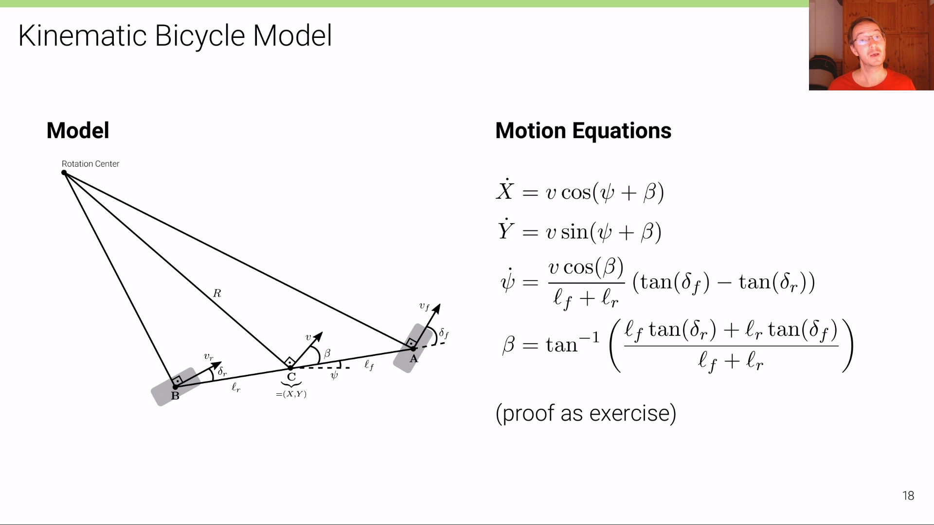
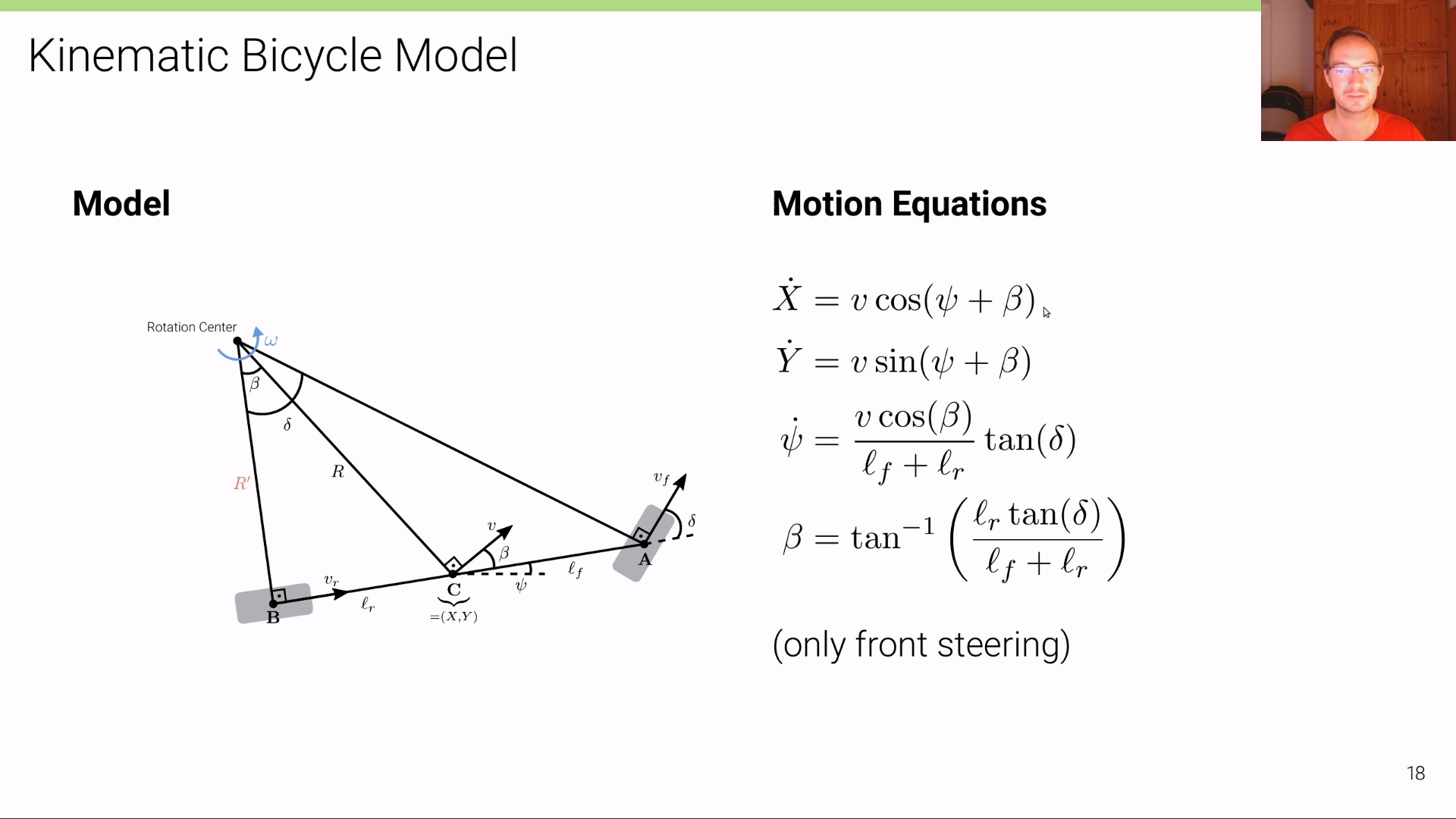
그러면 앞의 17 페이지의 정보를 이용하여 위 슬라이드와 같이 Motion Equation을 정의해 보겠습니다. \(\dot{X}, \dot{Y}, \dot{\psi}\) 는 각각 시간에 대하여 미분한 값을 의미하므로 \(X, Y, \psi\) 방향으로의 속도를 의미합니다.
먼저 \(X, Y\) 각 방향으로의 속도를 알기 위하여 삼각함수를 이용해 각 방향의 속도 성분을 구합니다. 따라서 Course Angle을 이용하여 각 방향의 속도는 다음과 같이 구할 수 있습니다.

\[\dot{X} = v \cos{\psi + \beta}\]
\[\dot{Y} = v \sin{\psi + \beta}\]

위 식에서 \(\psi\) 와 \(\beta\) 는 다소 복잡한 식으로 표현됩니다. 본 강의에서는 위 식을 좀 더 단순화 시켜서 살펴볼 예정입니다.

실제로 대부분의 차량의 경우 전륜만 회전을 하고 후륜은 전륜의 회전에 따라 움직이게 됩니다. 따라서 전륜과 후륜을 모두 모델링에 고려하기 보다 위 그림처럼 전륜만 고려 (only front steering)하면 모델을 단순화 시킬 수 있습니다.
위 그림과 같이 전륜만 고려하여 모델을 단순화 하면 바퀴의 회전도 \(\delta\) 하나만 고려할 수 있습니다.
그러면 전륜만 고려하였을 때, \(\dot{\psi}\) 와 \(\beta\) 를 어떻게 유도하는 지 살펴보도록 하겠습니다.

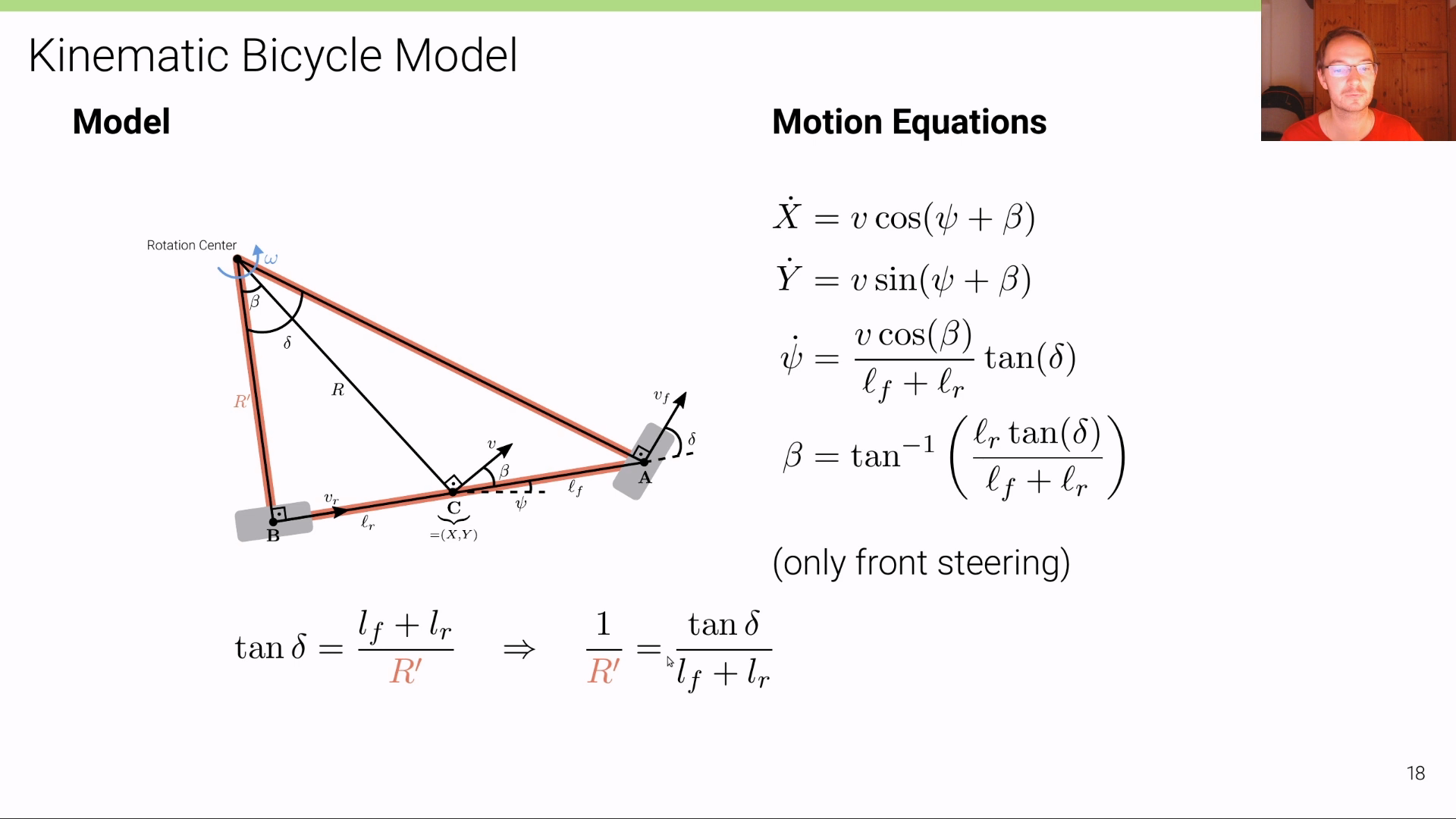
먼저 위 그림과 같이 빨간색 테두리의 삼각형 전체의 삼각 함수를 이용하면 다음 식을 도출할 수 있습니다.

\[\tan{\delta} = \frac{l_{f} + l_{r}}{R'}\]

식을 정리하면 다음과 같습니다.

\[\frac{1}{R'} = \frac{\tan{\delta}}{l_{f} + l_{r}}\]

위 그림의 빨간색 테두리의 삼각형의 끼인각인 \(\beta\) 와 앞에서 정리한 \(\frac{1}{R'}\) 를 이용하면 식을 다음과 같이 정리할 수 있습니다.

\[\tan{\beta} = \frac{l_{r}}{R'} = \frac{l_{r} \tan{\delta}}{l_{f} + l_{r}}\]
\[\therefore \beta = \tan^{-1}{(\frac{l_{r} \tan{\delta}}{l_{f} + l_{r}})}\]

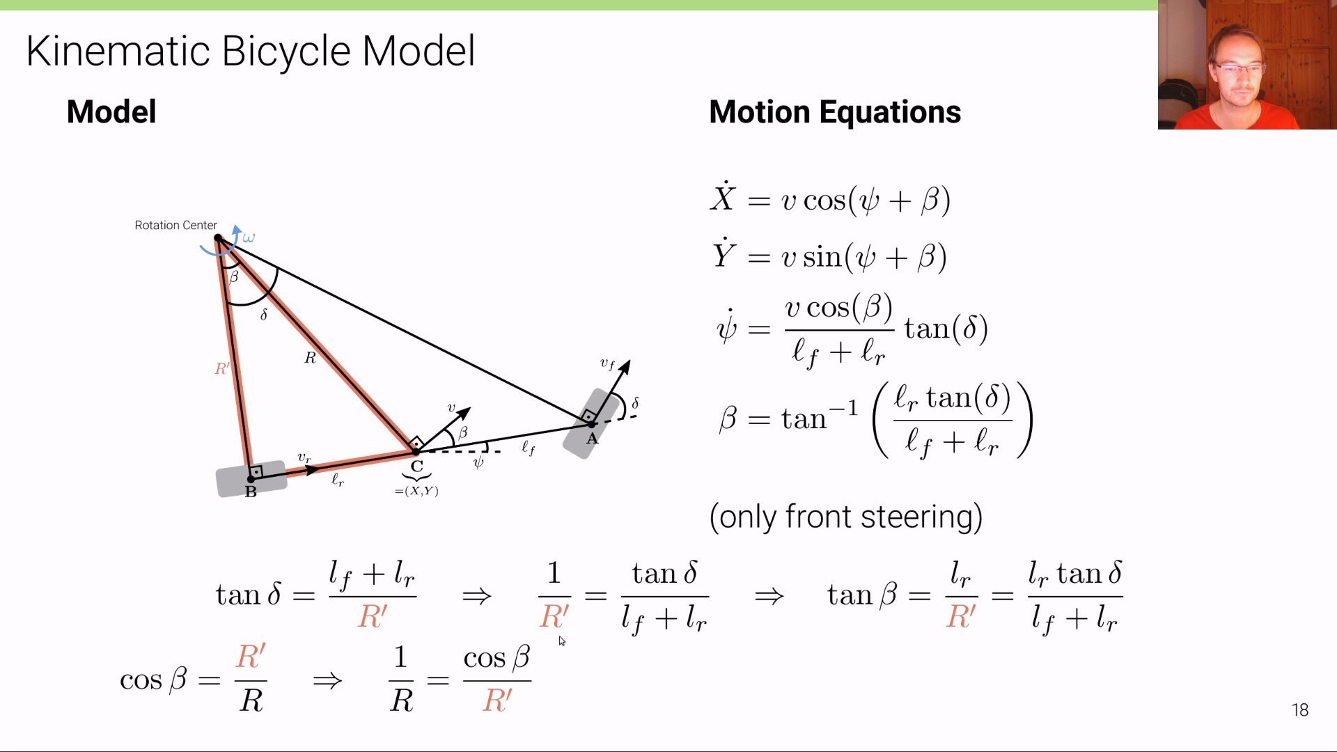
위 그림의 빨간색 테두리의 삼각형을 이용하여 다음과 같이 식을 정리할 수 있습니다. 이 값은 \(\dot{\psi}\) 를 유도할 때 사용합니다.

\[\cos{\beta} = \frac{R'}{R}\]
\[\frac{1}{R} = \frac{\cos{\beta}}{R'}\]

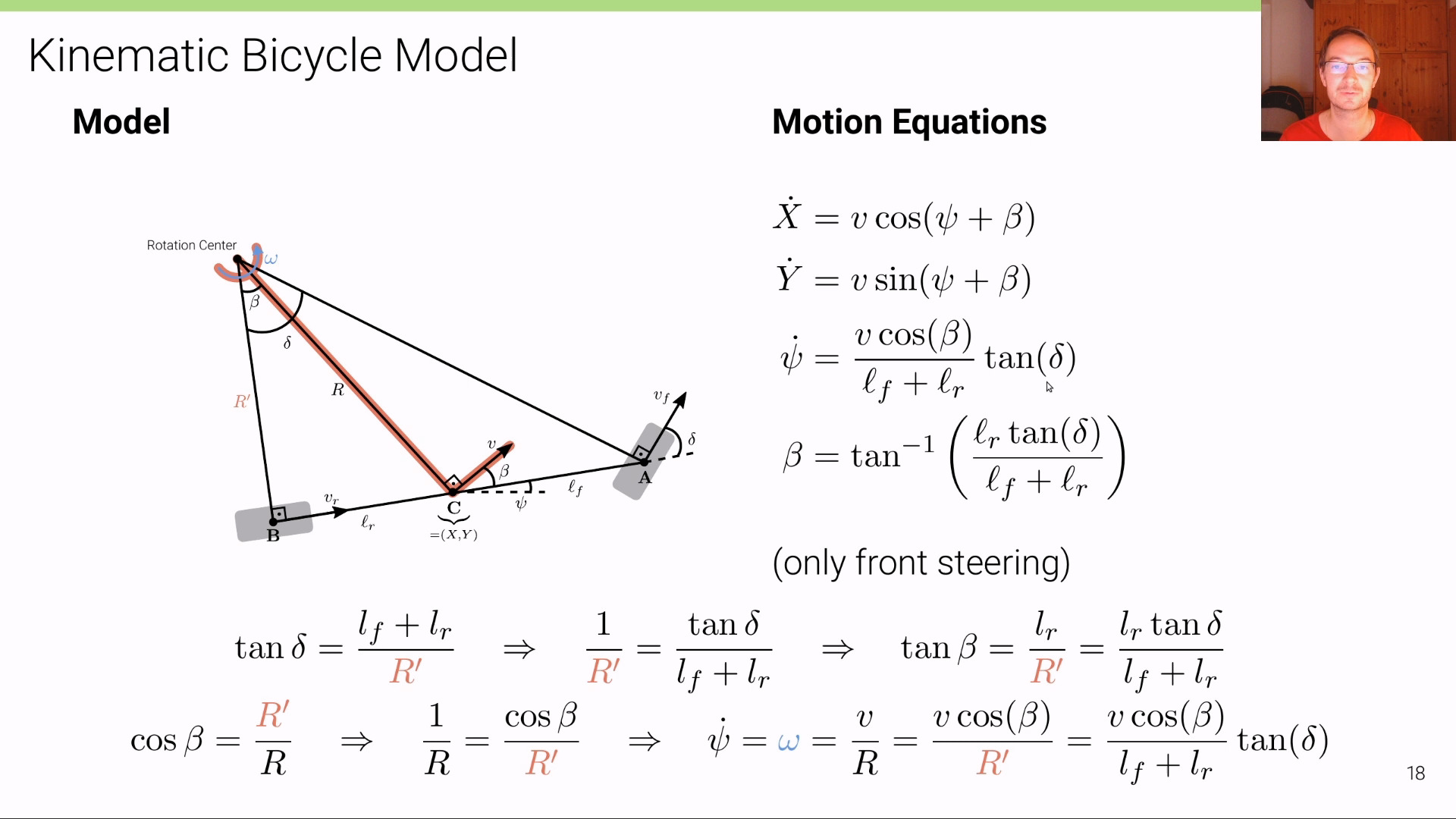
위 슬라이드와 같이 \(\dot{\psi}\) 는 차량의 각속도를 의미합니다. 각속도 \(\omega\) 는 반경과 반경에 직교하는 속도를 이용하여 구할 수 있습니다. 따라서 다음 조건을 이용해야 합니다.

\[\omega = \frac{v}{R} = \frac{v_{r}}{R'}\]

이 관계와 앞에서 정리한 \(\frac{1}{R}\) 를 이용하면 다음과 같이 \(\dot{\psi}\) 를 유도할 수 있습니다.

\[\dot{\psi} = \omega = \frac{v}{R} = \frac{v\cos{(\beta)}}{R'} = \frac{v\cos{(\beta)}}{l_{f} + l_{r}}\tan{(\delta)}\]

위 슬라이드에 나와있는 \(\dot{X}, \dot{Y}, \dot{\psi}, \beta\) 를 이용하여 Motion Equation을 정의해 볼 예정입니다. (글 조금 더 아래 내려보면 식과 코드를 정리하였습니다.)
만약 \(\beta\) 와 \(\delta\) 가 작은 경우라면 식이 좀 더 단순화 될 수 있습니다. 이 경우 차량이 단순 직진하는 경우에 해당합니다. 아래 슬라이드를 살펴보겠습니다.

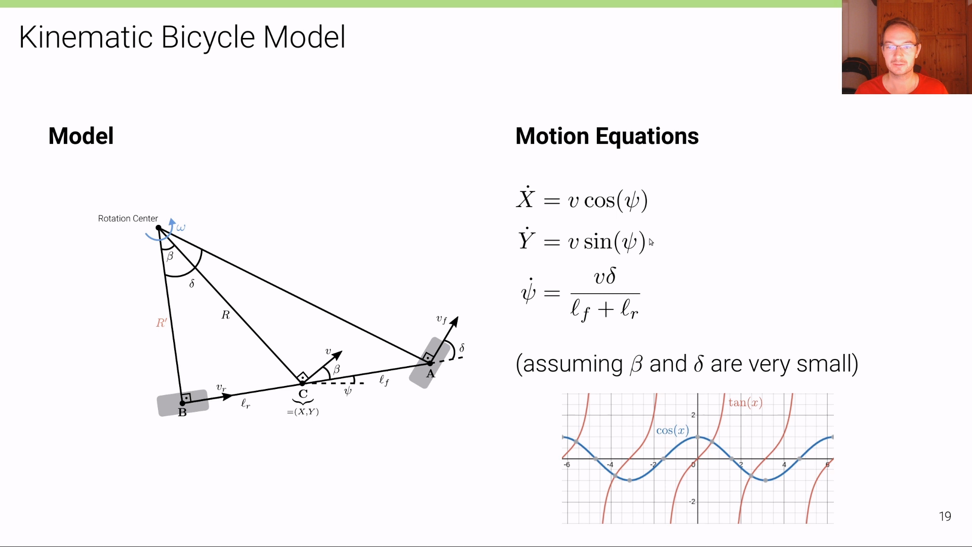
위 슬라이드는 \(\beta\) 가 극도로 작아져 0 인 경우를 가정하였습니다. 따라서 \(\beta\) 값은 소거되었습니다.
그리고 \(\delta\) 또한 작은 값이라면 \(\delta \approx \tan{(\delta)}\) 로 가정하여 위 슬라이드와 같이 간소화할 수 있습니다.

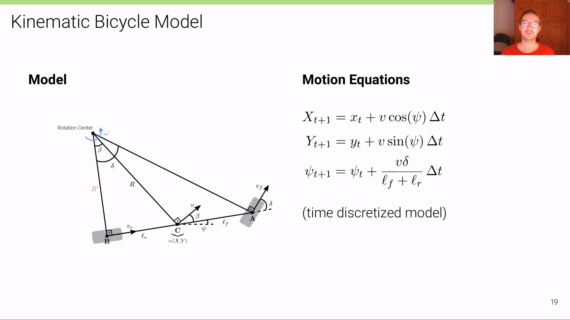
간소화된 버전을 이용하여 식을 정의하면 위 슬라이드와 같습니다. 하지만 위 식은 직진으로 이동하는 경우에만 고려될 수 있으므로 다음과 같이 \(\beta, \delta\) 를 모두 고려한 다음 식으로 점화식을 새워보면 다음과 같습니다.

\[X_{t+1} = X_{t} + v\cos{(\psi + \beta)}\Delta t\]
\[Y_{t+1} = Y_{t} + v\sin{(\psi + \beta)}\Delta t\]
\[\beta = \tan^{-1}{(\frac{l_{r} \tan{\delta}}{l_{f} + l_{r}})}\]
\[\psi_{t+1} = \psi_{t} + \frac{v \cos{(\beta)}}{l_{f} + l_{r}}\tan{(\delta)}\Delta t\]

아래 코드는 위 식을 기준으로 Kinematic Bicycle Model을 정의한 내용입니다.
initialize parameters에서 L, lr, dt는 실제 차량 환경을 고려한 길이를 넣어주어야 합니다.
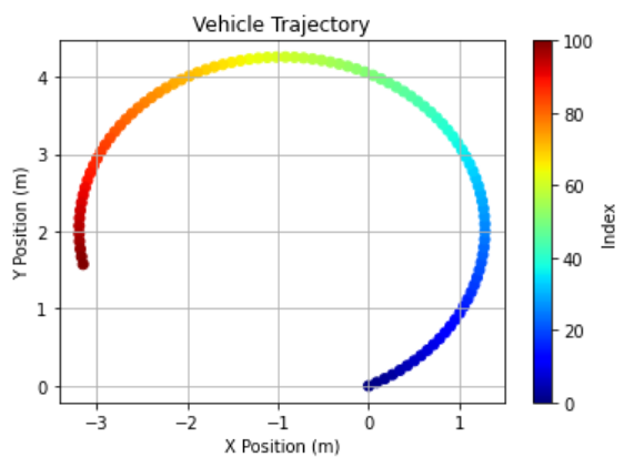
아래 코드의 constant inputs으로 정의한 v 와 delta 또한 실제 차량의 움직임의 센서값들을 넣어야 정상 동작합니다. 아래 코드는 고정된 \(v = 1 \text{ m/s}\) 와 \(\delta = 45 \text{ deg}\) 를 사용하였을 때의 차량의 이동 궤적을 구한 결과입니다.
차량의 위치 \(x, y\) 좌표는 차량의 무게 중심을 의미합니다.

import numpy as np
import matplotlib.pyplot as plt

# Initialize parameters
L = 2.0  # Wheelbase length
lr = 1.0  # Distance from center of mass to the rear axle
dt = 0.1  # Time step (s)
T = 10.0  # Total simulation time (s)
N = int(T / dt)  # Number of time steps

# Initialize state variables
x = np.zeros(N+1)
y = np.zeros(N+1)
psi = np.zeros(N+1)

# Initial conditions
x[0] = 0.0
y[0] = 0.0
psi[0] = 0.0

# Constant inputs for this example
# Velocity (m/s)
velocities = [1.0] * 100
# Steering angle (rad)
deltas = [np.pi / 4] * 100

# Time-discretized equations of motion
for t, (v, delta) in enumerate(zip(velocities, deltas)):
    beta = np.arctan((lr / L) * np.tan(delta))
    x[t + 1] = x[t] + dt * v * np.cos(psi[t] + beta)
    y[t + 1] = y[t] + dt * v * np.sin(psi[t] + beta)
    psi[t + 1] = psi[t] + dt * (v / L) * np.cos(beta) * np.tan(delta)

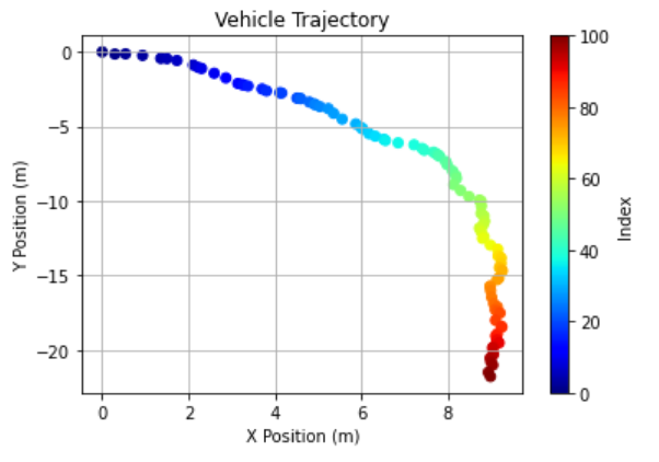
다음은 jet colormap으로 차량의 이동 궤적을 표현한 결과입니다. 인덱스의 색을 참조하면 파란색 부근이 시작점이고 빨간색 부근이 도착지점입니다.

# Plotting the trajectory
colors = np.arange(len(x))
# Create scatter plot with color gradation
plt.scatter(x, y, c=colors, cmap='jet')
plt.grid(True)
plt.colorbar(label='Index')
plt.xlabel('X Position (m)')
plt.ylabel('Y Position (m)')
plt.title('Vehicle Trajectory')
plt.show()

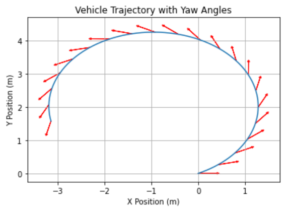
아래는 이동 경로의 회전을 표현하기 위하여 \(\psi\) 각도를 화살표로 시각화 하여 표현한 결과입니다.

이번에는 \(v\) 와 \(\delta\) 에 임의의 값을 지정하여 한번 그려보겠습니다.
\(v\) 는 5 m/s 이하의 속도의 랜덤값이고 \(\delta\) 는 18도 ~ 45도 각도의 랜덤 값입니다.

import numpy as np
import matplotlib.pyplot as plt

# Initialize parameters
L = 2.0  # Wheelbase length
lr = 1.0  # Distance from center of mass to the rear axle
dt = 0.1  # Time step (s)
T = 10.0  # Total simulation time (s)
N = int(T / dt)  # Number of time steps

# Initialize state variables
x = np.zeros(N+1)
y = np.zeros(N+1)
psi = np.zeros(N+1)

# Initial conditions
x[0] = 0.0
y[0] = 0.0
psi[0] = 0.0

# Constant inputs for this example
# Velocity (m/s)
velocities = [random.random()*5 for _ in range(N)]
# Steering angle (rad)
deltas = [(-1)**(random.randint(0, 1))*(np.pi/random.randint(4, 10)) for _ in range(N)]

# Time-discretized equations of motion
for t, (v, delta) in enumerate(zip(velocities, deltas)):
    beta = np.arctan((lr / L) * np.tan(delta))
    x[t + 1] = x[t] + dt * v * np.cos(psi[t] + beta)
    y[t + 1] = y[t] + dt * v * np.sin(psi[t] + beta)
    psi[t + 1] = psi[t] + dt * (v / L) * np.cos(beta) * np.tan(delta)

# Plotting the trajectory
colors = np.arange(len(x))

# Create scatter plot with color gradation
plt.scatter(x, y, c=colors, cmap='jet')
plt.grid(True)
plt.colorbar(label='Index')
plt.xlabel('X Position (m)')
plt.ylabel('Y Position (m)')
plt.title('Vehicle Trajectory')
plt.show()

# Function to plot arrow
def plot_arrow(x, y, yaw, length=0.7, width=0.2):
    plt.arrow(x, y, length * np.cos(yaw), length * np.sin(yaw),
              head_length=width, head_width=width, fc='r', ec='r')

# Plotting the trajectory
plt.figure()
plt.plot(x, y)

# Plot arrows to indicate psi (yaw angle)
arrow_interval = 3
for i in range(0, len(psi), arrow_interval):
    plot_arrow(x[i], y[i], psi[i])


plt.xlabel('X Position (m)')
plt.ylabel('Y Position (m)')
plt.title('Vehicle Trajectory with Yaw Angles')
plt.grid(True)
plt.show()

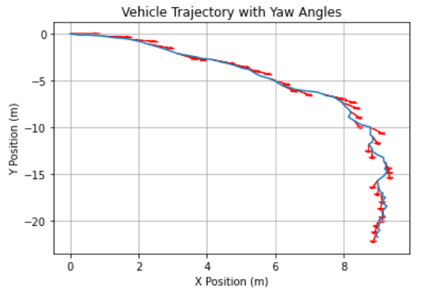
따라서 위 그림과 같이 차속 \(v\) 와 앞 바퀴의 회전 각도 \(\delta\) 를 알 수 있으면 차량의 이동 궤적을 구할 수 있음을 확인할 수 있었습니다.

만약 앞에서 구한 \(x, y\) 의 위치 이동과 \(\psi\) 를 이용하여 3차원 상의 Rotation과 Translation을 구한다면 다음과 같습니다.

def get_transformation_matrix(x, y, z, psi):
    R = np.array([[np.cos(psi), -np.sin(psi), 0],
                  [np.sin(psi), np.cos(psi), 0],
                  [0, 0, 1]])
    
    t = np.array([x, y, z]).reshape(3, 1)
    
    T = np.hstack([R, t])
    T = np.vstack([T, [0, 0, 0, 1]])
    
    return T

# Example usage
x, y, z = 1.0, 2.0, 0.0  # x, y, and z coordinates
psi = np.pi / 4  # yaw angle in radians

T = get_transformation_matrix(x, y, z, psi)
print("3D Transformation Matrix:")
print(T)

# 3D Transformation Matrix:
# [[ 0.70710678 -0.70710678  0.          1.        ]
#  [ 0.70710678  0.70710678  0.          2.        ]
#  [ 0.          0.          1.          0.        ]
#  [ 0.          0.          0.          1.        ]]​

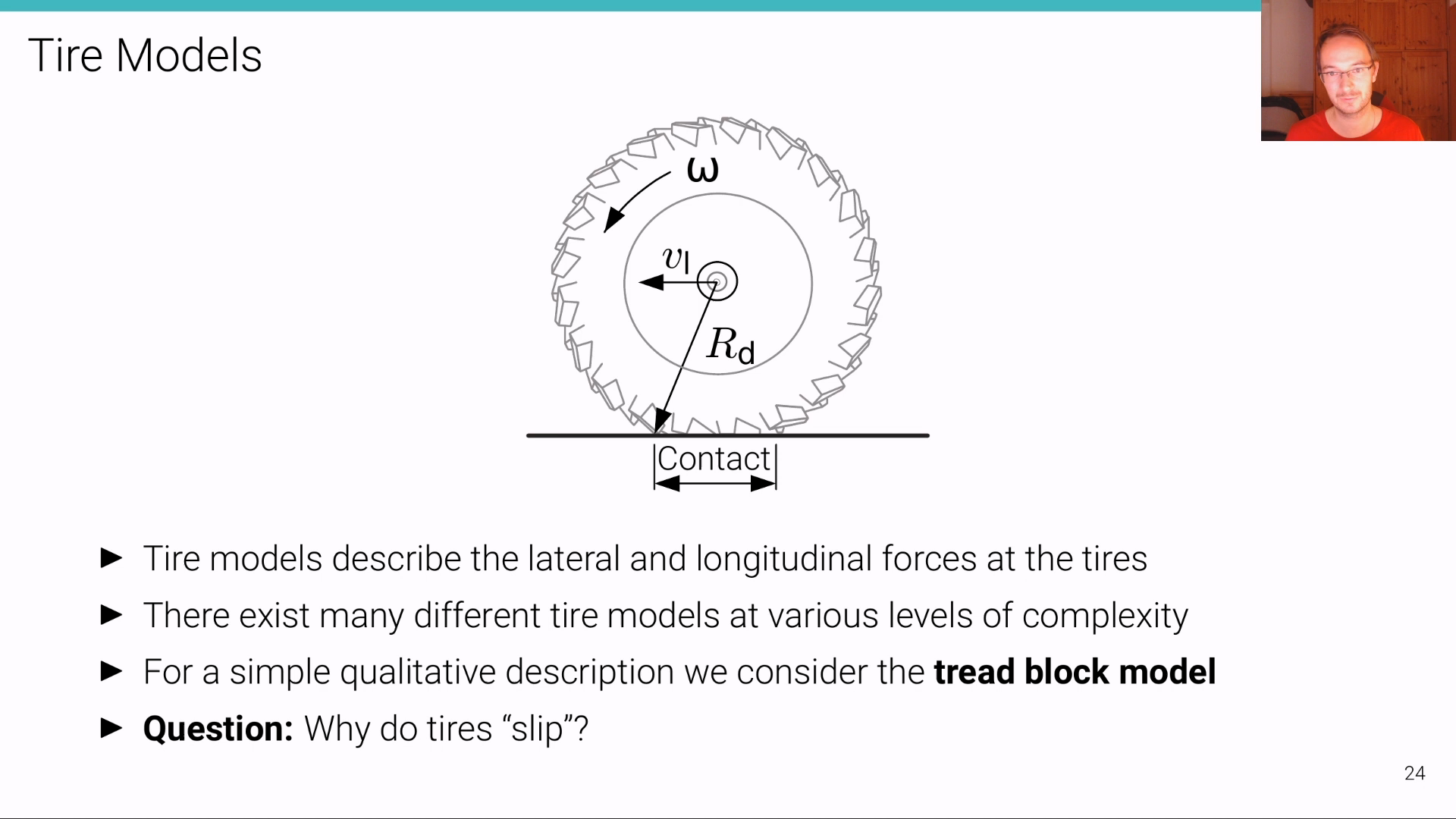
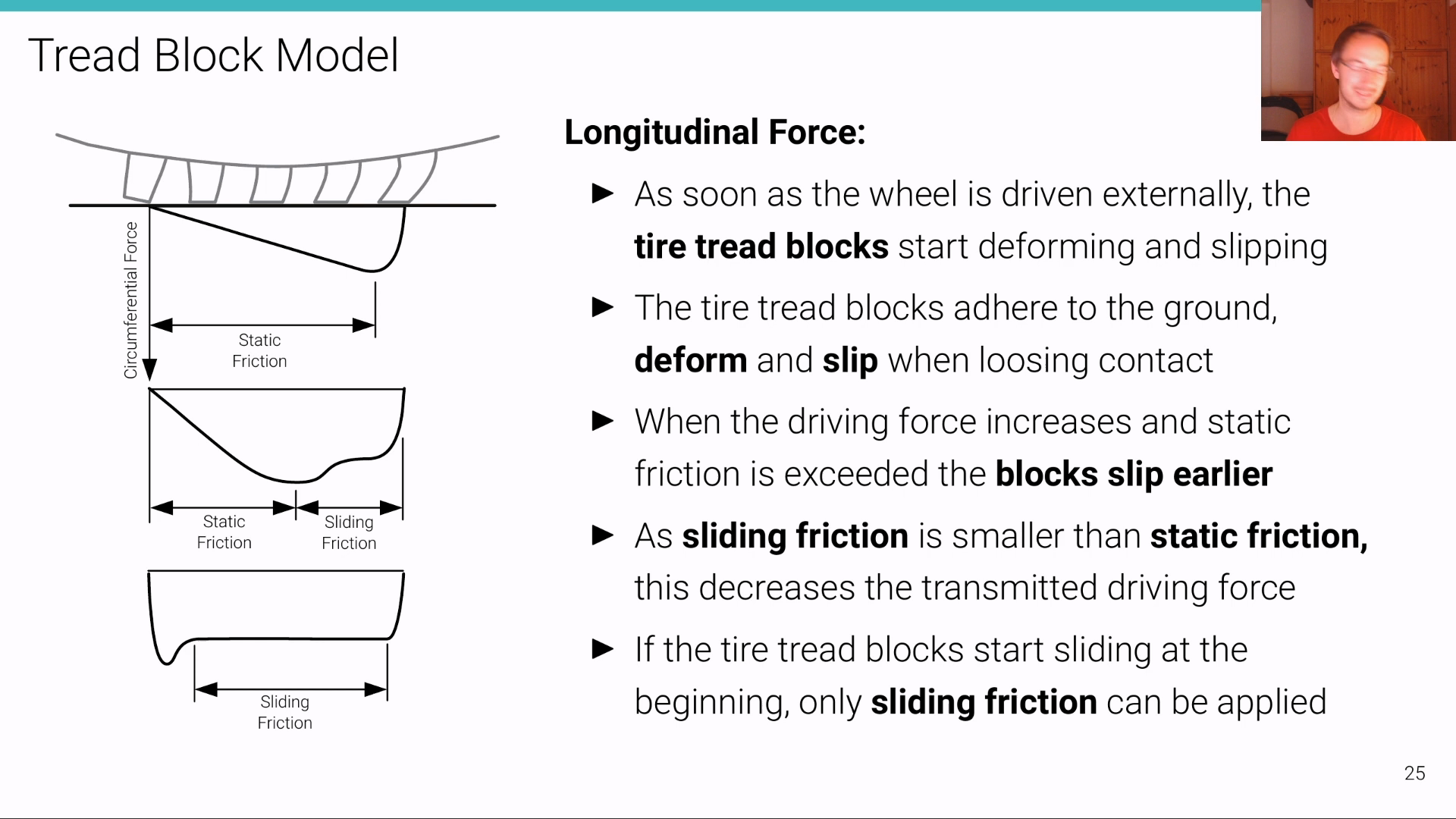
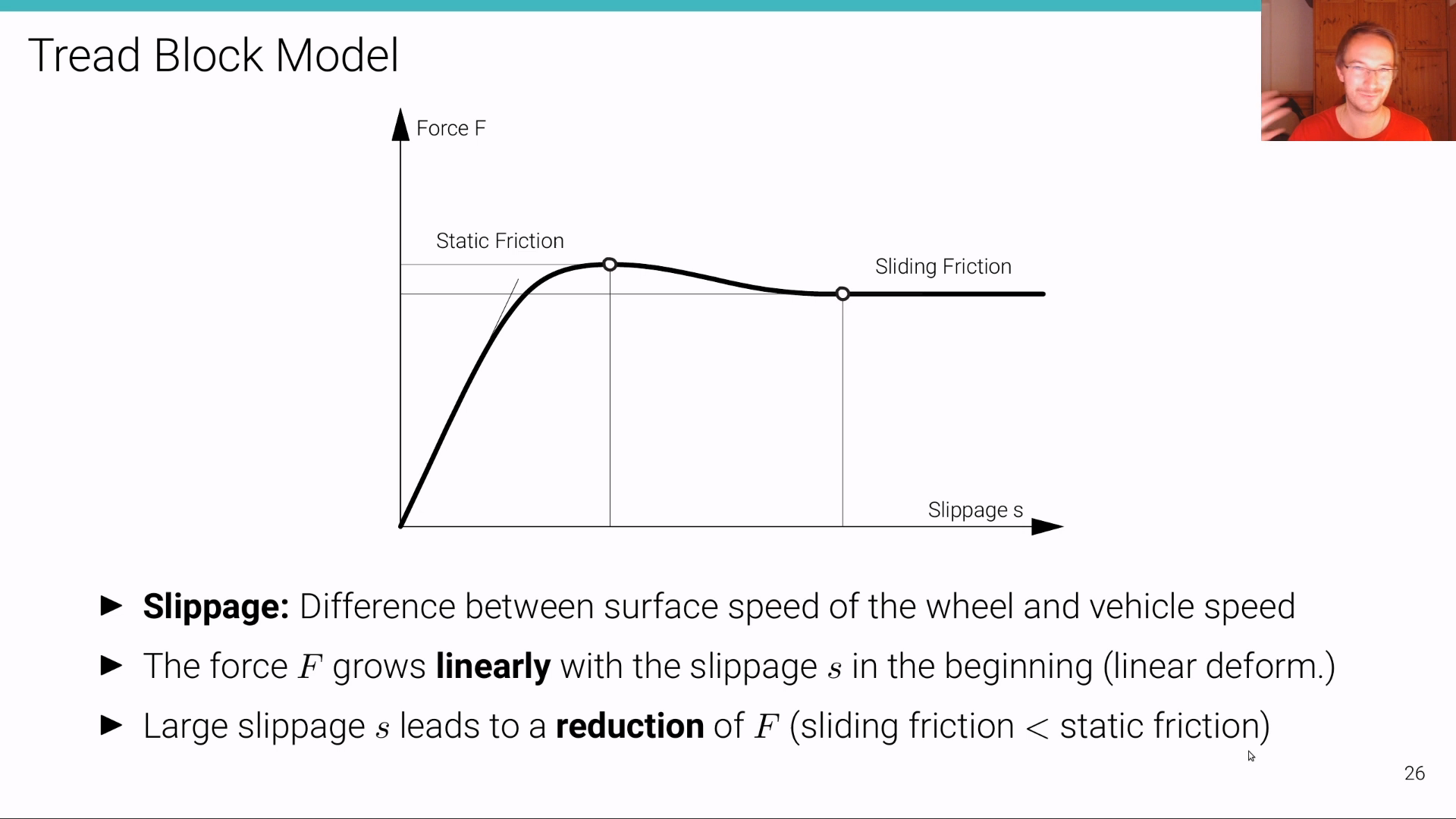
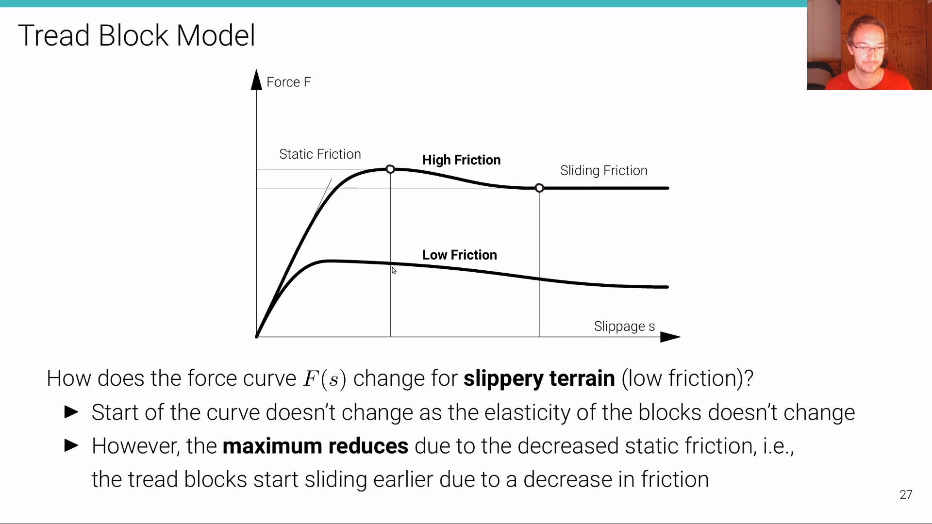
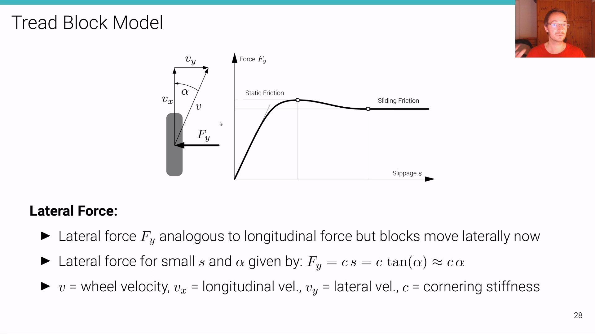
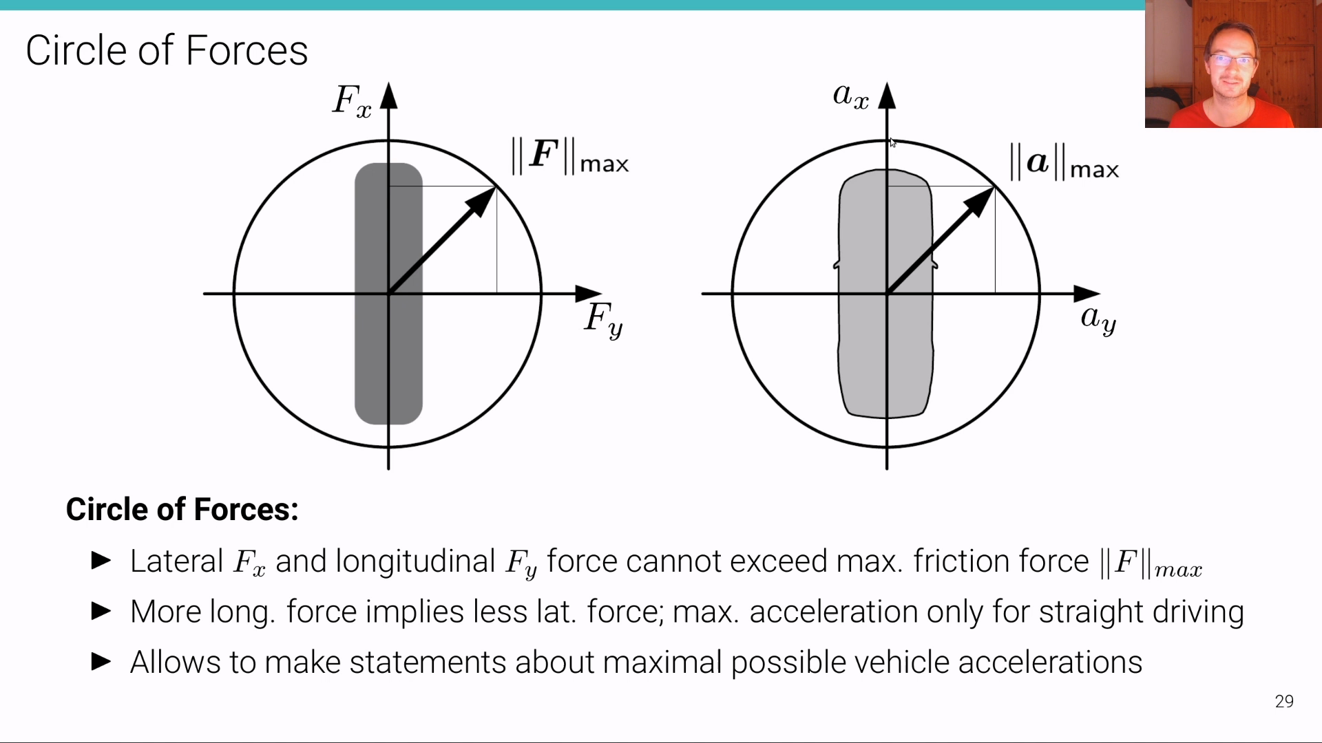
Tire Models

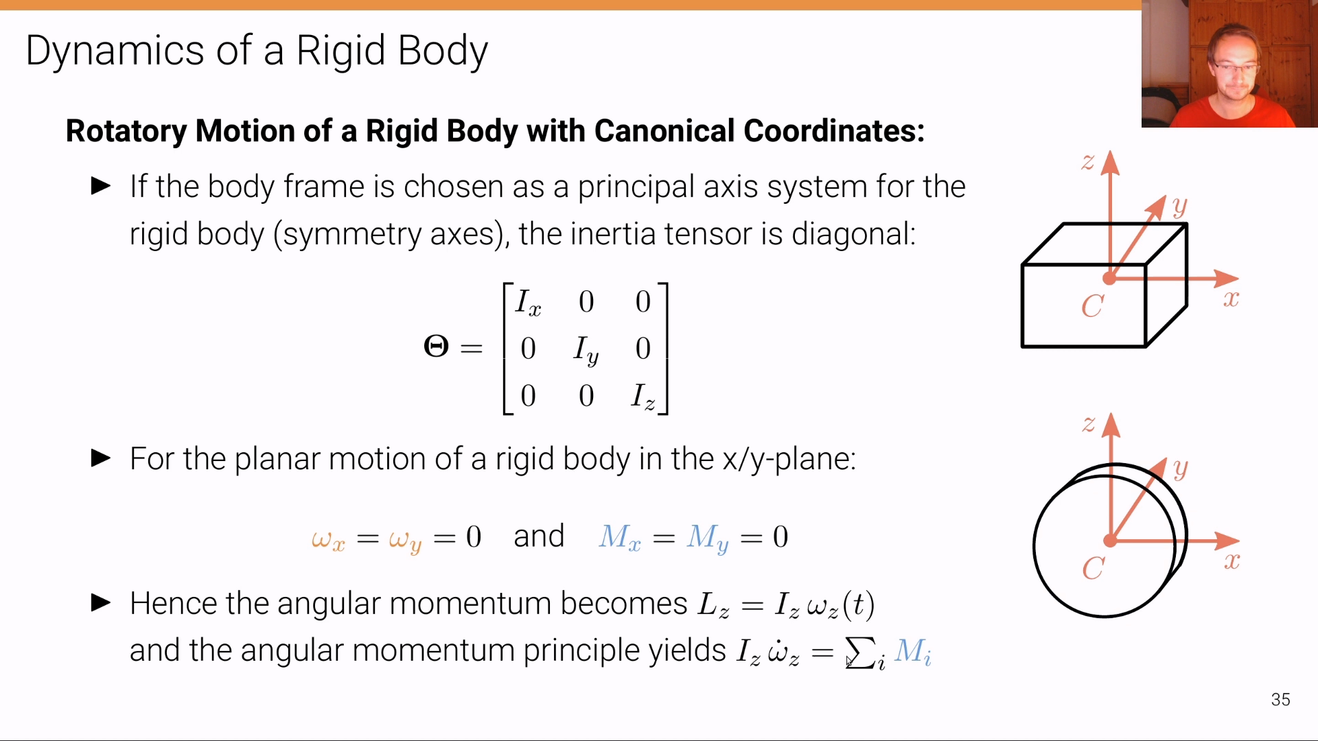
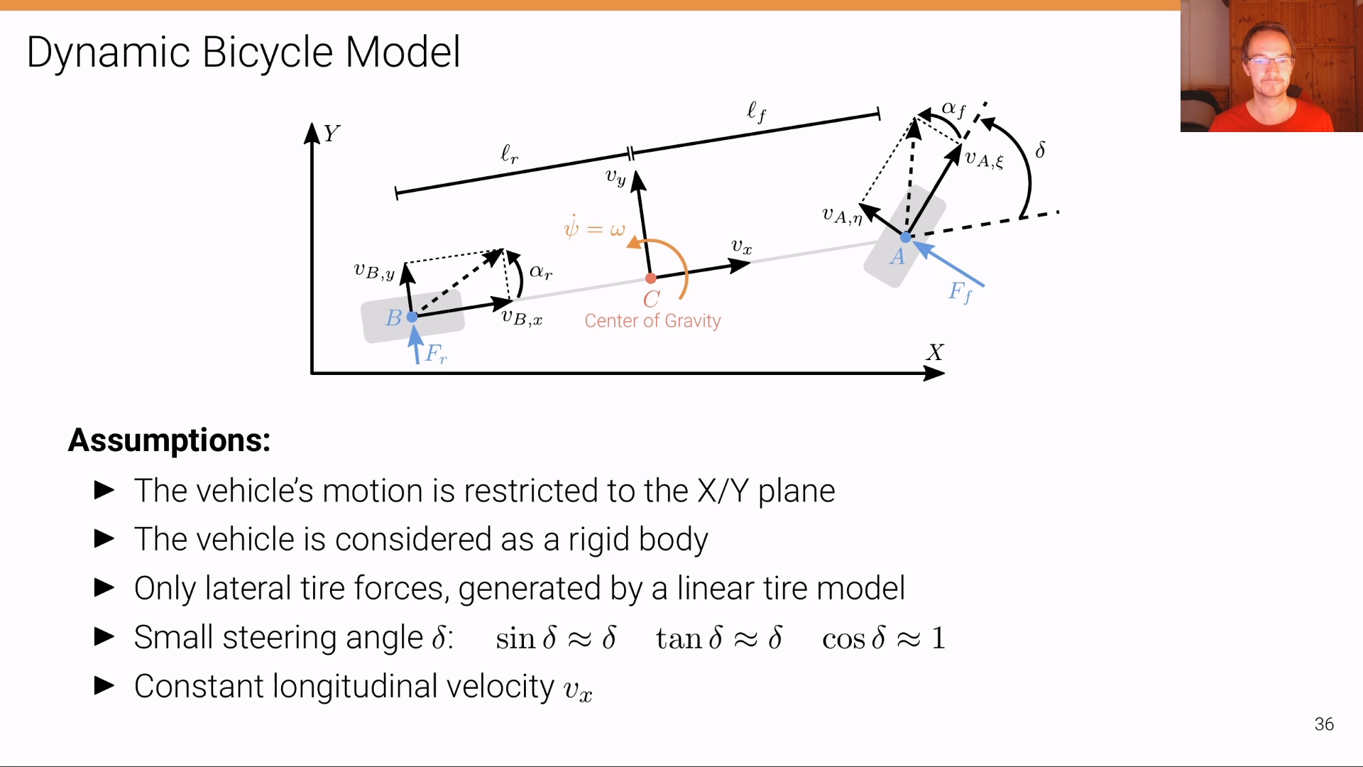
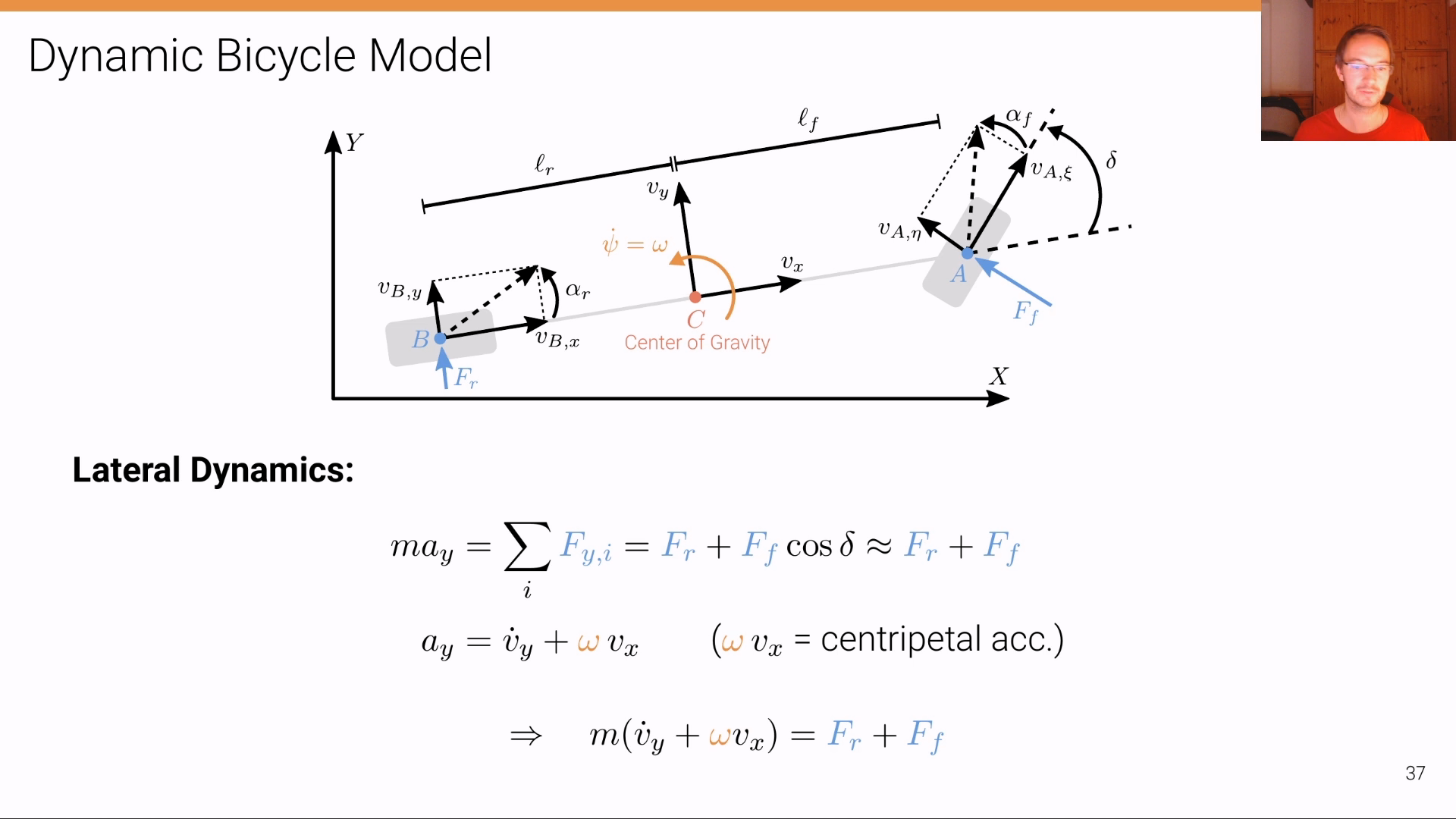
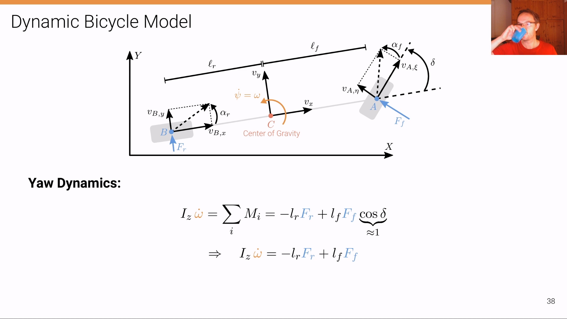
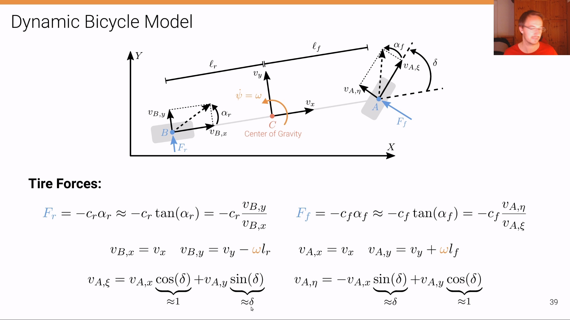
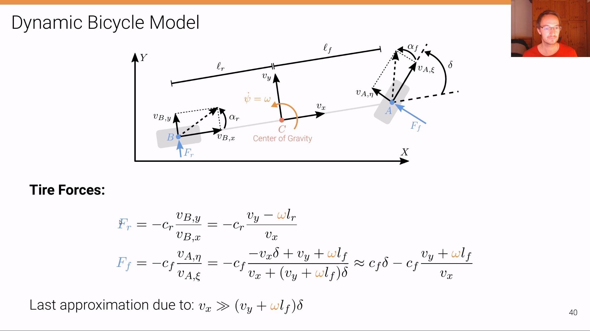
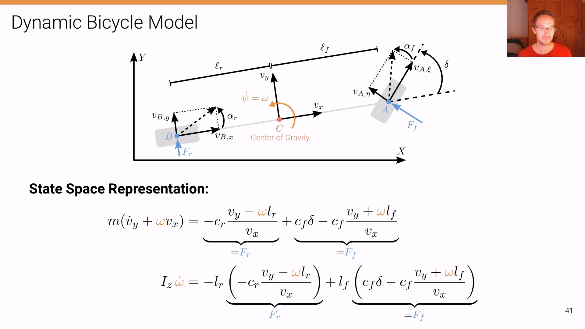
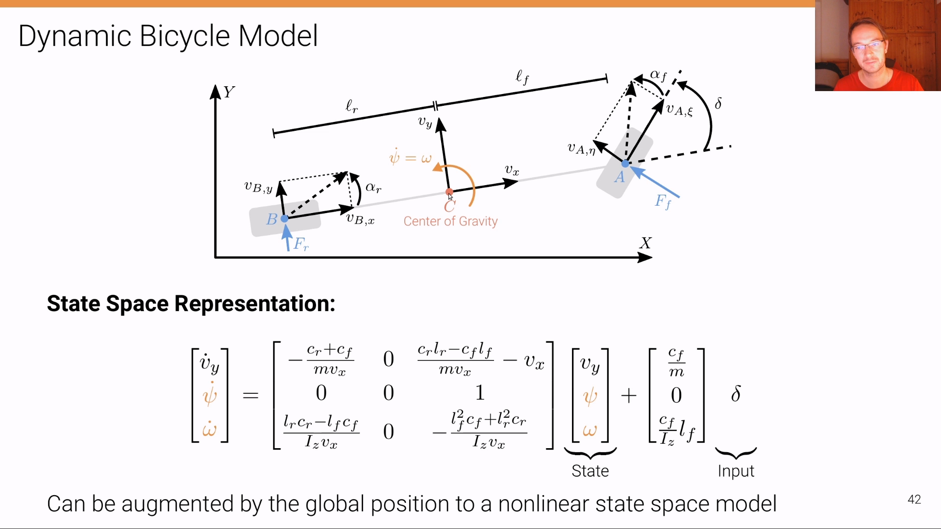
Dynamic Bicycle Model

Optimal State Estimation 글 목차