5-1. Deep learning for computer vision, Introduction to convnets

This chapter (Deep learning for computer vision) covers

• Understanding convolutional neural networks (convnets)
• Using data augmentation to mitigate overfitting
• Using a pretrained convnet to do feature extraction
• Fine-tuning a pretrained convnet
• Visualizing what convnets learn and how they make classification decisions

5.1 Introduction to convnets

The following lines of code show you what a basic convnet looks like.
It’s a stack of Conv2D and MaxPooling2D layers. You’ll see in a minute exactly what they do.

• Instantiating a small convnet

model = models.Sequential()
model.add(layers.Conv2D(32, (3, 3), activation='relu', input_shape=(28, 28, 1)))
model.add(layers.MaxPooling2D((2, 2)))
model.add(layers.Conv2D(64, (3, 3), activation='relu'))
model.add(layers.MaxPooling2D((2, 2)))
model.add(layers.Conv2D(64, (3, 3), activation='relu'))

A convnet takes as input tensors of shape (image_height, image_width, image_channels). In this case, we’ll configure the convnet to process inputs of size (28, 28, 1), which is the format of MNIST images. We’ll do this by passing the argument input_shape=(28, 28, 1) to the first layer.

>>> model.summary()
________________________________________________________________
Layer (type)                     Output Shape          Param #
================================================================
conv2d_1 (Conv2D)                (None, 26, 26, 32)    320
________________________________________________________________
maxpooling2d_1 (MaxPooling2D)    (None, 13, 13, 32)    0
________________________________________________________________
conv2d_2 (Conv2D)                (None, 11, 11, 64)    18496
________________________________________________________________
maxpooling2d_2 (MaxPooling2D)    (None, 5, 5, 64)      0
________________________________________________________________
conv2d_3 (Conv2D)                (None, 3, 3, 64)      36928
================================================================
Total params: 55,744
Trainable params: 55,744
Non-trainable params: 0

You can see that the output of every Conv2D and MaxPooling2D layer is a 3D tensor of shape (height, width, channels). The width and height dimensions tend to shrink as you go deeper in the network. The number of channels is controlled by the first argument passed to the Conv2D layers (32 or 64).

The next step is to feed the last output tensor (of shape (3, 3, 64)) into a densely connected classifier network like those you’re already familiar with: a stack of Dense layers. These classifiers process vectors, which are 1D, whereas the current output is a 3D tensor. First we have to flatten the 3D outputs to 1D, and then add a few Dense layers on top.

• Adding a classifier on top of the convnet

model.add(layers.Flatten())
model.add(layers.Dense(64, activation='relu'))
model.add(layers.Dense(10, activation='softmax'))

We’ll do 10-way classification, using a final layer with 10 outputs and a softmax activation. Here’s what the network looks like now:

>>> model.summary()
Layer (type)                     Output Shape          Param #
================================================================
conv2d_1 (Conv2D)                (None, 26, 26, 32)    320
________________________________________________________________
maxpooling2d_1 (MaxPooling2D)    (None, 13, 13, 32)    0
________________________________________________________________
conv2d_2 (Conv2D)                (None, 11, 11, 64)    18496
________________________________________________________________
maxpooling2d_2 (MaxPooling2D)    (None, 5, 5, 64)      0
________________________________________________________________
conv2d_3 (Conv2D)                (None, 3, 3, 64)      36928
________________________________________________________________
flatten_1 (Flatten)              (None, 576)           0
________________________________________________________________
dense_1 (Dense)                  (None, 64)            36928
________________________________________________________________
dense_2 (Dense)                  (None, 10)            650
================================================================
Total params: 93,322
Trainable params: 93,322
Non-trainable params: 0

As you can see, the (3, 3, 64) outputs are flattened into vectors of shape (576,) before going through two Dense layers. Now, let’s train the convnet on the MNIST digits.

• Training the convnet on MNIST images

from keras.datasets import mnist
from keras.utils import to_categorical

(train_images, train_labels), (test_images, test_labels) = mnist.load_data()
train_images = train_images.reshape((60000, 28, 28, 1))
train_images = train_images.astype('float32') / 255

test_images = test_images.reshape((10000, 28, 28, 1))
test_images = test_images.astype('float32') / 255

train_labels = to_categorical(train_labels)
test_labels = to_categorical(test_labels)

model.compile(optimizer='rmsprop',
              loss='categorical_crossentropy',
              metrics=['accuracy'])
model.fit(train_images, train_labels, epochs=5, batch_size=64)

Let’s evaluate the model on the test data:

>>> test_loss, test_acc = model.evaluate(test_images, test_labels)
>>> test_acc
0.99080000000000001

why does this simple convnet work so well, compared to a densely connected model? To answer this, let’s dive into what the Conv2D and MaxPooling2D layers do.

5.1.1 The convolution operation

The fundamental difference between a densely connected layer and a convolution layer is this:

Dense layers learn global patterns in their input feature space (for example, for a MNIST digit, patterns involving all pixels), whereas convolution layers learn local patterns

in the case of images, patterns found in small 2D windows of the inputs. In the previous example, these windows were all 3 × 3.

• Images can be broken into local patterns such as edges, textures, and so on.

• This key characteristic gives convnets two interesting properties:

  • The patterns they learn are translation invariant. After learning a certain pattern in the lower-right corner of a picture, a convnet can recognize it anywhere: for example, in the upper-left corner. A densely connected network would have to learn the pattern anew if it appeared at a new location. This makes convnets data efficient when processing images (because the visual world is fundamentally translation invariant): they need fewer training samples to learn representations that have generalization power.

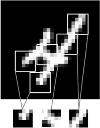
  • They can learn spatial hierarchies of patterns (see, below). A first convolution layer will learn small local patterns such as edges, a second convolution layer will learn larger patterns made of the features of the first layers, and so on. This allows convnets to efficiently learn increasingly complex and abstract visual concepts (because the visual world is fundamentally spatially hierarchical).

• The visual world forms a spatial hierarchy of visual modules: hyperlocal edges combine into local objects such as eyes or ears, which combine into high-level concepts such as “cat.”

Convolutions operate over 3D tensors, called feature maps, with two spatial axes (height and width) as well as a depth axis (also called the channels axis). For an RGB image, the dimension of the depth axis is 3, because the image has three color channels: red, green, and blue : red, green, and blue. For a black-and-white picture, like the MNIST digits, the depth is 1 (levels of gray). The convolution operation extracts patches from its input feature map and applies the same transformation to all of these patches, producing an output feature map. This output feature map is still a 3D tensor: it has a width and a height. Its depth can be arbitrary, because the output depth is a parameter of the layer, and the different channels in that depth axis no longer stand for specific colors as in RGB input; rather, they stand for filters. Filters encode specific aspects of the input data: at a high level, a single filter could encode the concept “presence of a face in the input,” for instance.

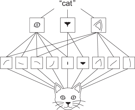
In the MNIST example, the first convolution layer takes a feature map of size (28, 28, 1) and outputs a feature map of size (26, 26, 32): it computes 32 filters over its input. Each of these 32 output channels contains a 26 × 26 grid of values, which is a response map of the filter over the input, indicating the response of that filter pattern at different locations in the input. (refer below) That is what the term feature map means: every dimension in the depth axis is a feature (or filter), and the 2D tensor output[:, :, n] is the 2D spatial map of the response of this filter over the input.

• The concept of a response map: a 2D map of the presence of a pattern at different locations in an input

• Convolutions are defined by two key parameters:
  • Size of the patches extracted from the inputs — These are typically 3 × 3 or 5 × 5. In the example, they were 3 × 3, which is a common choice.
  • Depth of the output feature map— The number of filters computed by the convolution. The example started with a depth of 32 and ended with a depth of 64.

In Keras Conv2D layers, these parameters are the first arguments passed to the layer: Conv2D(output_depth, (window_height, window_width)).

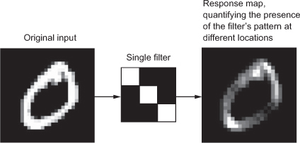
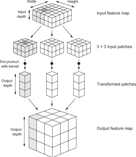
A convolution works by sliding these windows of size 3 × 3 or 5 × 5 over the 3D input feature map, stopping at every possible location, and extracting the 3D patch of surrounding features (shape (window_height, window_width, input_depth)). Each such 3D patch is then transformed (via a tensor product with the same learned weight matrix, called the convolution kernel) into a 1D vector of shape (output_depth,). Every spatial location in the output feature map corresponds to the same location in the input feature map (for example, the lower-right corner of the output contains information about the lower-right corner of the input). For instance, with 3 × 3 windows, the vector output[i, j, :] comes from the 3D patch input[i-1:i+1, j-1:j+1, :]. The full process is detailed below.

• How convolution works

Note that the output width and height may differ from the input width and height. They may differ for two reasons:

• Border effects, which can be countered by padding the input feature map
• The use of strides, which I’ll define in a second

Let’s take a deeper look at these notions

Understanding border effects and padding

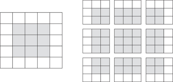
Consider a 5 × 5 feature map (25 tiles total). There are only 9 tiles around which you can center a 3 × 3 window, forming a 3 × 3 grid. Hence, the output feature map will be 3 × 3. It shrinks a little: by exactly two tiles alongside each dimension, in this case.v You can see this border effect in action in the earlier example: you start with 28 × 28 inputs, which become 26 × 26 after the first convolution layer.

• Valid locations of 3 × 3 patches in a 5 × 5 input feature map

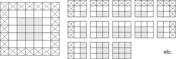
If you want to get an output feature map with the same spatial dimensions as the input, you can use padding. Padding consists of adding an appropriate number of rows and columns on each side of the input feature map so as to make it possible to fit center convolution windows around every input tile. For a 3 × 3 window, you add one column on the right, one column on the left, one row at the top, and one row at the bottom. For a 5 × 5 window, you add two rows.

• Padding a 5 × 5 input in order to be able to extract 25 3 × 3 patches

In Conv2D layers, padding is configurable via the padding argument, which takes two values:

• valid : which means no padding (only valid window locations will be used)
• same : which means “pad in such a way as to have an output with the same width and height as the input.

The padding argument defaults to "valid".

Understanding convolution strides

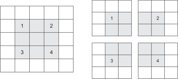
The other factor that can influence output size is the notion of strides. The description of convolution so far has assumed that the center tiles of the convolution windows are all contiguous. But the distance between two successive windows is a parameter of the convolution, called its stride, which defaults to 1. It’s possible to have strided convolutions: convolutions with a stride higher than 1. you can see the patches extracted by a 3 × 3 convolution with stride 2 over a 5 × 5 input (without padding).

• 3 × 3 convolution patches with 2 × 2 strides

Using stride 2 means the width and height of the feature map are downsampled by a factor of 2 (in addition to any changes induced by border effects). Strided convolutions are rarely used in practice, although they can come in handy for some types of models; it’s good to be familiar with the concept.

To downsample feature maps, instead of strides, we tend to use the max-pooling operation, which you saw in action in the first convnet example. Let’s look at it in more depth.

5.1.2 The max-pooling operation

In the convnet example, you may have noticed that the size of the feature maps is halved after every MaxPooling2D layer. For instance, before the first MaxPooling2D layers, the feature map is 26 × 26, but the max-pooling operation halves it to 13 × 13. That’s the role of max pooling: to aggressively downsample feature maps, much like strided convolutions.

Max pooling consists of extracting windows from the input feature maps and outputting the max value of each channel. It’s conceptually similar to convolution, except that instead of transforming local patches via a learned linear transformation (the convolution kernel), they’re transformed via a hardcoded max tensor operation. A big difference from convolution is that max pooling is usually done with 2 × 2 windows and stride 2, in order to downsample the feature maps by a factor of 2. On the other hand, convolution is typically done with 3 × 3 windows and no stride (stride 1).

Why downsample feature maps this way? Why not remove the max-pooling layers and keep fairly large feature maps all the way up? Let’s look at this option. The convolutional base of the model would then look like this:

model_no_max_pool = models.Sequential()
model_no_max_pool.add(layers.Conv2D(32, (3, 3), activation='relu',
                      input_shape=(28, 28, 1)))
model_no_max_pool.add(layers.Conv2D(64, (3, 3), activation='relu'))
model_no_max_pool.add(layers.Conv2D(64, (3, 3), activation='relu'))

Here’s a summary of the model:

>>> model_no_max_pool.summary()

Layer (type)                     Output Shape          Param #
================================================================
conv2d_4 (Conv2D)                (None, 26, 26, 32)    320
________________________________________________________________
conv2d_5 (Conv2D)                (None, 24, 24, 64)    18496
________________________________________________________________
conv2d_6 (Conv2D)                (None, 22, 22, 64)    36928
================================================================
Total params: 55,744
Trainable params: 55,744
Non-trainable params: 0

What’s wrong with this setup? Two things:

• It isn’t conducive to learning a spatial hierarchy of features. The 3 × 3 windows in the third layer will only contain information coming from 7 × 7 windows in the initial input. The high-level patterns learned by the convnet will still be very small with regard to the initial input, which may not be enough to learn to classify digits (try recognizing a digit by only looking at it through windows that are 7 × 7 pixels!). We need the features from the last convolution layer to contain information about the totality of the input.
• The final feature map has 22 × 22 × 64 = 30,976 total coefficients per sample. This is huge. If you were to flatten it to stick a Dense layer of size 512 on top, that layer would have 15.8 million parameters. This is far too large for such a small model and would result in intense overfitting.

In short, the reason to use downsampling is

• to reduce the number of feature-map coefficients to process
• to induce spatial-filter hierarchies by making successive convolution layers look at increasingly large windows (in terms of the fraction of the original input they cover).

Note that max pooling isn’t the only way you can achieve such downsampling. As you already know, you can also use strides in the prior convolution layer. And you can use average pooling instead of max pooling, where each local input patch is transformed by taking the average value of each channel over the patch, rather than the max. But max pooling tends to work better than these alternative solutions. In a nutshell, the reason is that features tend to encode the spatial presence of some pattern or concept over the different tiles of the feature map (hence, the term feature map), and it’s more informative to look at the maximal presence of different features than at their average presence. So the most reasonable subsampling strategy is to first produce dense maps of features (via unstrided convolutions) and then look at the maximal activation of the features over small patches, rather than looking at sparser windows of the inputs (via strided convolutions) or averaging input patches, which could cause you to miss or dilute feature-presence information.

At this point, you should understand the basics of convnets—feature maps, convolution, and max pooling—and you know how to build a small convnet to solve a toy problem such as MNIST digits classification. Now let’s move on to more useful, practical applications.