5-2. Training a convnet from scratch on a small dataset

Having to train an image-classification model using very little data is a common situation, which you’ll likely encounter in practice if you ever do computer vision in a professional context. A “few” samples can mean anywhere from a few hundred to a few tens of thousands of images. As a practical example, we’ll focus on classifying images as dogs or cats, in a dataset containing 4,000 pictures of cats and dogs (2,000 cats, 2,000 dogs). We’ll use 2,000 pictures for training—1,000 for validation, and 1,000 for testing.

In this section, we’ll review one basic strategy to tackle this problem:
training a new model from scratch using what little data you have. You’ll start by naively training a small convnet on the 2,000 training samples, without any regularization, to set a baseline for what can be achieved. This will get you to a classification accuracy of 71%. At that point, the main issue will be overfitting. Then we’ll introduce data augmentation, a powerful technique for mitigating overfitting in computer vision. By using data augmentation, you’ll improve the network to reach an accuracy of 82%.

In the next section, we’ll review two more essential techniques for applying deep learning to small datasets:
feature extraction with a pretrained network (which will get you to an accuracy of 90% to 96%) and fine-tuning a pretrained network (this will get you to a final accuracy of 97%). Together, these three strategies—

• training a small model from scratch
• doing feature extraction using a pretrained model
• fine-tuning a pretrained model

will constitute your future toolbox for tackling the problem of performing image classification with small datasets.

5.2.1. The relevance of deep learning for small-data problems

You’ll sometimes hear that deep learning only works when lots of data is available. This is valid in part: one fundamental characteristic of deep learning is that it can find interesting features in the training data on its own, without any need for manual feature engineering, and this can only be achieved when lots of training examples are available. This is especially true for problems where the input samples are very high-dimensional, like images.

But what constitutes lots of samples is relative—relative to the size and depth of the network you’re trying to train, for starters. It isn’t possible to train a convnet to solve a complex problem with just a few tens of samples, but a few hundred can potentially suffice if the model is small and well regularized and the task is simple. Because convnets learn local, translation-invariant features, they’re highly data efficient on perceptual problems. Training a convnet from scratch on a very small image dataset will still yield reasonable results despite a relative lack of data, without the need for any custom feature engineering. You’ll see this in action in this section.

What’s more, deep-learning models are by nature highly repurposable: you can take, say, an image-classification or speech-to-text model trained on a large-scale dataset and reuse it on a significantly different problem with only minor changes. Specifically, in the case of computer vision, many pretrained models (usually trained on the Image-Net dataset) are now publicly available for download and can be used to bootstrap powerful vision models out of very little data. That’s what you’ll do in the next section. Let’s start by getting your hands on the data.

5.2.2. Downloading the data

The Dogs vs. Cats dataset that you’ll use isn’t packaged with Keras. It was made available by Kaggle as part of a computer-vision competition in late 2013, back when convnets weren’t mainstream. You can download the original dataset from www.kaggle.com/c/dogs-vs-cats/data

The pictures are medium-resolution color JPEGs.

• Samples from the Dogs vs. Cats dataset. Sizes weren’t modified: the samples are heterogeneous in size, appearance, and so on.

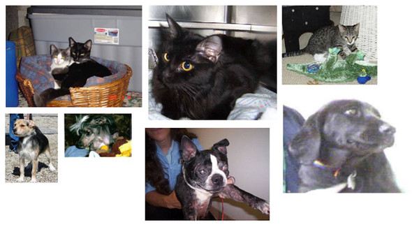
Unsurprisingly, the dogs-versus-cats Kaggle competition in 2013 was won by entrants who used convnets. The best entries achieved up to 95% accuracy. In this example, you’ll get fairly close to this accuracy (in the next section), even though you’ll train your models on less than 10% of the data that was available to the competitors.

This dataset contains 25,000 images of dogs and cats (12,500 from each class) and is 543 MB (compressed). After downloading and uncompressing it, you’ll create a new dataset containing three subsets: a training set with 1,000 samples of each class, a validation set with 500 samples of each class, and a test set with 500 samples of each class.

After uncompressing data, Directory structure is below.(Before run below code, cats_and_dogs_small is empty)

├───cats_and_dogs_small
│   ├───test
│   │   ├───cats
│   │   └───dogs
│   ├───train
│   │   ├───cats
│   │   └───dogs
│   └───validation
│       ├───cats
│       └───dogs
├───test1
└───train

• Copying images to training, validation, and test directories

import os, shutil

# Path to the directory where the original dataset was uncompressed
original_dataset_dir = './train'

# Directory where you’ll store your smaller dataset
base_dir = './cats_and_dogs_small'
os.mkdir(base_dir)

# Directories for the training, validation, and test splits
train_dir = os.path.join(base_dir, 'train')
os.mkdir(train_dir)
validation_dir = os.path.join(base_dir, 'validation')
os.mkdir(validation_dir)
test_dir = os.path.join(base_dir, 'test')
os.mkdir(test_dir)

# Directory with training cat pictures
train_cats_dir = os.path.join(train_dir, 'cats')
os.mkdir(train_cats_dir)

# Directory with training dog pictures
train_dogs_dir = os.path.join(train_dir, 'dogs')
os.mkdir(train_dogs_dir)

# Directory with validation cat pictures
validation_cats_dir = os.path.join(validation_dir, 'cats')
os.mkdir(validation_cats_dir)

# Directory with validation dog pictures
validation_dogs_dir = os.path.join(validation_dir, 'dogs')
os.mkdir(validation_dogs_dir)

# Directory with test cat pictures
test_cats_dir = os.path.join(test_dir, 'cats')
os.mkdir(test_cats_dir)

# Directory with test dog pictures
test_dogs_dir = os.path.join(test_dir, 'dogs')
os.mkdir(test_dogs_dir)

# Copies the first 1,000 cat images to train_cats_dir
fnames = ['cat.{}.jpg'.format(i) for i in range(1000)]
for fname in fnames:
    src = os.path.join(original_dataset_dir, fname)
    dst = os.path.join(train_cats_dir, fname)
    shutil.copyfile(src, dst)

# Copies the next 500 cat images to validation_cats_dir
fnames = ['cat.{}.jpg'.format(i) for i in range(1000, 1500)]
for fname in fnames:
    src = os.path.join(original_dataset_dir, fname)
    dst = os.path.join(validation_cats_dir, fname)
    shutil.copyfile(src, dst)

# Copies the next 500 cat images to test_cats_dir
fnames = ['cat.{}.jpg'.format(i) for i in range(1500, 2000)]
for fname in fnames:
    src = os.path.join(original_dataset_dir, fname)
    dst = os.path.join(test_cats_dir, fname)
    shutil.copyfile(src, dst)

# Copies the first 1,000 dog images to train_dogs_dir
fnames = ['dog.{}.jpg'.format(i) for i in range(1000)]
for fname in fnames:
    src = os.path.join(original_dataset_dir, fname)
    dst = os.path.join(train_dogs_dir, fname)
    shutil.copyfile(src, dst)

# Copies the next 500 dog images to validation_dogs_dir 
fnames = ['dog.{}.jpg'.format(i) for i in range(1000, 1500)]
for fname in fnames:
    src = os.path.join(original_dataset_dir, fname)
    dst = os.path.join(validation_dogs_dir, fname)
    shutil.copyfile(src, dst)

# Copies the next 500 dog images to test_dogs_dir
fnames = ['dog.{}.jpg'.format(i) for i in range(1500, 2000)]
for fname in fnames:
    src = os.path.join(original_dataset_dir, fname)
    dst = os.path.join(test_dogs_dir, fname)
    shutil.copyfile(src, dst)

As a sanity check, let’s count how many pictures are in each training split (train/validation/test):

>>> print('total training cat images:', len(os.listdir(train_cats_dir)))
total training cat images: 1000
>>> print('total training dog images:', len(os.listdir(train_dogs_dir)))
total training dog images: 1000
>>> print('total validation cat images:', len(os.listdir(validation_cats_dir)))
total validation cat images: 500
>>> print('total validation dog images:', len(os.listdir(validation_dogs_dir)))
total validation dog images: 500
>>> print('total test cat images:', len(os.listdir(test_cats_dir)))
total test cat images: 500
>>> print('total test dog images:', len(os.listdir(test_dogs_dir)))
total test dog images: 500

So you do indeed have 2,000 training images, 1,000 validation images, and 1,000 test images. Each split contains the same number of samples from each class: this is a balanced binary-classification problem, which means classification accuracy will be an appropriate measure of success.

5.2.3. Building your network

You built a small convnet for MNIST in the previous example, so you should be familiar with such convnets. You’ll reuse the same general structure: the convnet will be a stack of alternated Conv2D (with relu activation) and MaxPooling2D layers.

But because you’re dealing with bigger images and a more complex problem, you’ll make your network larger, accordingly: it will have one more Conv2D + MaxPooling2D stage. This serves both to augment the capacity of the network and to further reduce the size of the feature maps so they aren’t overly large when you reach the Flatten layer. Here, because you start from inputs of size 150 × 150 (a somewhat arbitrary choice), you end up with feature maps of size 7 × 7 just before the Flatten layer.

The depth of the feature maps progressively increases in the network (from 32 to 128), whereas the size of the feature maps decreases (from 128 × 128 to 7 × 7). This is a pattern you’ll see in almost all convnets.

Because you’re attacking a binary-classification problem, you’ll end the network with a single unit (a Dense layer of size 1) and a sigmoid activation. This unit will encode the probability that the network is looking at one class or the other.

• Instantiating a small convnet for dogs vs. cats classification

from keras import layers
from keras import models

model = models.Sequential()
model.add(layers.Conv2D(32, (3, 3), activation='relu',
                        input_shape=(150, 150, 3)))
model.add(layers.MaxPooling2D((2, 2)))
model.add(layers.Conv2D(64, (3, 3), activation='relu'))
model.add(layers.MaxPooling2D((2, 2)))
model.add(layers.Conv2D(128, (3, 3), activation='relu'))
model.add(layers.MaxPooling2D((2, 2)))
model.add(layers.Conv2D(128, (3, 3), activation='relu'))
model.add(layers.MaxPooling2D((2, 2)))
model.add(layers.Flatten())
model.add(layers.Dense(512, activation='relu'))
model.add(layers.Dense(1, activation='sigmoid'))

Let’s look at how the dimensions of the feature maps change with every successive layer:

>>> model.summary()
Layer (type)                     Output Shape          Param #
================================================================
conv2d_1 (Conv2D)                (None, 148, 148, 32)  896
________________________________________________________________
maxpooling2d_1 (MaxPooling2D)    (None, 74, 74, 32)    0
________________________________________________________________
conv2d_2 (Conv2D)                (None, 72, 72, 64)    18496
________________________________________________________________
maxpooling2d_2 (MaxPooling2D)    (None, 36, 36, 64)    0
________________________________________________________________
conv2d_3 (Conv2D)                (None, 34, 34, 128)   73856
________________________________________________________________
maxpooling2d_3 (MaxPooling2D)    (None, 17, 17, 128)   0
________________________________________________________________
conv2d_4 (Conv2D)                (None, 15, 15, 128)   147584
________________________________________________________________
maxpooling2d_4 (MaxPooling2D)    (None, 7, 7, 128)     0
________________________________________________________________
flatten_1 (Flatten)              (None, 6272)          0
________________________________________________________________
dense_1 (Dense)                  (None, 512)           3211776
________________________________________________________________
dense_2 (Dense)                  (None, 1)             513
================================================================
Total params: 3,453,121
Trainable params: 3,453,121
Non-trainable params: 0

For the compilation step, you’ll go with the RMSprop optimizer, as usual. Because you ended the network with a single sigmoid unit, you’ll use binary crossentropy as the loss

• Configuring the model for training ```python from keras import optimizers

model.compile(loss=’binary_crossentropy’, optimizer=optimizers.RMSprop(lr=1e-4), metrics=[‘acc’])

<br>

### 5.2.4. Data preprocessing

As you know by now, data should be formatted into appropriately preprocessed floating-point tensors before being fed into the network. 
Currently, the data sits on a drive as JPEG files, so the steps for getting it into the network are roughly as follows:

1. Read the picture files.
2. Decode the JPEG content to RGB grids of pixels.
3. Convert these into floating-point tensors.
4. Rescale the pixel values (between 0 and 255) to the [0, 1] interval (as you know, neural networks prefer to deal with small input values).

It may seem a bit daunting, but fortunately Keras has utilities to take care of these steps automatically. Keras has a module with image-processing helper tools, located at `keras.preprocessing.image`.
In particular, it contains the class `ImageDataGenerator`, which lets you quickly set up Python generators that can automatically turn image files on disk into batches of preprocessed tensors.
This is what you’ll use here.

+ Using ImageDataGenerator to read images from directories
```python
from keras.preprocessing.image import ImageDataGenerator

train_datagen = ImageDataGenerator(rescale=1./255)
test_datagen = ImageDataGenerator(rescale=1./255)

train_generator = train_datagen.flow_from_directory(
        train_dir,
        target_size=(150, 150)
        batch_size=20,
        class_mode='binary')

validation_generator = test_datagen.flow_from_directory(
        validation_dir,
        target_size=(150, 150),
        batch_size=20,
        class_mode='binary')

UNDERSTANDING PYTHON GENERATORS

A Python generator is an object that acts as an iterator: it’s an object you can use with the for ... in operator. Generators are built using the yield operator.

def generator():
    i = 0
    while True:
        i += 1
        yield i

for item in generator():
    print(item)
    if item > 4:
        break

It prints this:

1 2 3 4 5

Let’s look at the output of one of these generators: it yields batches of 150 × 150 RGB images (shape (20, 150, 150, 3)) and binary labels (shape (20,)). There are 20 samples in each batch (the batch size). Note that the generator yields these batches indefinitely: it loops endlessly over the images in the target folder. For this reason, you need to break the iteration loop at some point:

>>> for data_batch, labels_batch in train_generator:
>>>     print('data batch shape:', data_batch.shape)
>>>     print('labels batch shape:', labels_batch.shape)
>>>     break
data batch shape: (20, 150, 150, 3)
labels batch shape: (20,)

Let’s fit the model to the data using the generator. You do so using the fit_generator method, the equivalent of fit for data generators like this one. It expects as its first argument a Python generator that will yield batches of inputs and targets indefinitely, like this one does. Because the data is being generated endlessly, the Keras model needs to know how many samples to draw from the generator before declaring an epoch over. This is the role of the steps_per_epoch argument: after having drawn steps_per_epoch batches from the generator —that is, after having run for steps_per_epoch gradient descent steps—the fitting process will go to the next epoch. In this case, batches are 20 samples, so it will take 100 batches until you see your target of 2,000 samples.

When using fit_generator, you can pass a validation_data argument, much as with the fit method. It’s important to note that this argument is allowed to be a data generator, but it could also be a tuple of Numpy arrays. If you pass a generator as validation_data, then this generator is expected to yield batches of validation data endlessly; hus you should also specify the validation_steps argument, which tells the process how many batches to draw from the validation generator for evaluation.

• Fitting the model using a batch generator

  history = model.fit_generator(
      train_generator,
      steps_per_epoch=100,
      epochs=30,
      validation_data=validation_generator,
      validation_steps=50)
  

  
  

It’s good practice to always save your models after training.

• Saving the model

model.save('cats_and_dogs_small_1.h5')

Let’s plot the loss and accuracy of the model over the training and validation data during training.

• Displaying curves of loss and accuracy during training

import matplotlib.pyplot as plt

acc = history.history['acc']
val_acc = history.history['val_acc']
loss = history.history['loss']
val_loss = history.history['val_loss']

epochs = range(1, len(acc) + 1)

plt.plot(epochs, acc, 'bo', label='Training acc')
plt.plot(epochs, val_acc, 'b', label='Validation acc')
plt.title('Training and validation accuracy')
plt.legend()

plt.figure()

plt.plot(epochs, loss, 'bo', label='Training loss')
plt.plot(epochs, val_loss, 'b', label='Validation loss')
plt.title('Training and validation loss')
plt.legend()

plt.show()

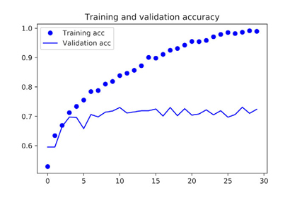
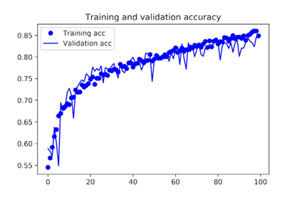
• Training and validation accuracy

• Training and validation loss

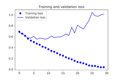
These plots are characteristic of overfitting. The training accuracy increases linearly over time, until it reaches nearly 100%, whereas the validation accuracy stalls at 70–72%. The validation loss reaches its minimum after only five epochs and then stalls, whereas the training loss keeps decreasing linearly until it reaches nearly 0.

Because you have relatively few training samples (2,000), overfitting will be your number-one concern. You already know about a number of techniques that can help mitigate overfitting, such as dropout and weight decay (L2 regularization). We’re now going to work with a new one, specific to computer vision and used almost universally when processing images with deep-learning models: data augmentation.

5.2.5. Using data augmentation

Overfitting is caused by having too few samples to learn from, rendering you unable to train a model that can generalize to new data. Given infinite data, your model would be exposed to every possible aspect of the data distribution at hand: you would never overfit. Data augmentation takes the approach of generating more training data from existing training samples, by augmenting the samples via a number of random transformations that yield believable-looking images. The goal is that at training time, your model will never see the exact same picture twice. This helps expose the model to more aspects of the data and generalize better.

In Keras, this can be done by configuring a number of random transformations to be performed on the images read by the ImageDataGenerator instance. Let’s get started with an example.

• Setting up a data augmentation configuration via ImageDataGenerator

datagen = ImageDataGenerator(
      rotation_range=40,
      width_shift_range=0.2,
      height_shift_range=0.2,
      shear_range=0.2,
      zoom_range=0.2,
      horizontal_flip=True,
      fill_mode='nearest')

These are just a few of the options available (for more, see the Keras documentation). Let’s quickly go over this code:

• rotation_range is a value in degrees (0–180), a range within which to randomly rotate pictures.
• width_shift and height_shift are ranges (as a fraction of total width or height) within which to randomly translate pictures vertically or horizontally.
• shear_range is for randomly applying shearing transformations.
• zoom_range is for randomly zooming inside pictures.
• horizontal_flip is for randomly flipping half the images horizontally—relevant when there are no assumptions of horizontal asymmetry (for example, real-world pictures).
• fill_mode is the strategy used for filling in newly created pixels, which can appear after a rotation or a width/height shift.

Let’s look at the augmented images

• Displaying some randomly augmented training images

# Module with image-preprocessing utilities
from keras.preprocessing import image

fnames = [os.path.join(train_cats_dir, fname) for
     fname in os.listdir(train_cats_dir)]

# Chooses one image to augment
img_path = fnames[3]

# Reads the image and resizes it
img = image.load_img(img_path, target_size=(150, 150))

# Converts it to a Numpy array with shape (150, 150, 3)
x = image.img_to_array(img)

# Reshapes it to (1, 150, 150, 3)
x = x.reshape((1,) + x.shape)

# Generates batches of randomly transformed images. 
# Loops indefinitely, so you need to break the loop at some point!
i = 0
for batch in datagen.flow(x, batch_size=1):
    plt.figure(i)
    imgplot = plt.imshow(image.array_to_img(batch[0]))
    i += 1
    if i % 4 == 0:
        break

plt.show()

• Generation of cat pictures via random data augmentation

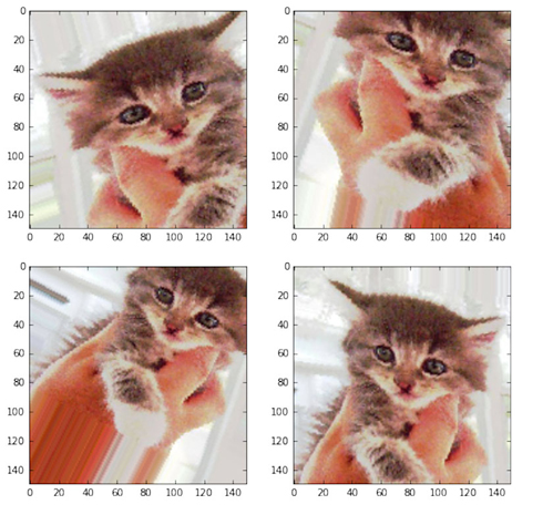
If you train a new network using this data-augmentation configuration, the network will never see the same input twice. But the inputs it sees are still heavily intercorrelated, because they come from a small number of original images— you can’t produce new information, you can only remix existing information. As such, this may not be enough to completely get rid of overfitting. To further fight overfitting, you’ll also add a Dropout layer to your model, right before the densely connected classifier.

• Defining a new convnet that includes dropout

model = models.Sequential()
model.add(layers.Conv2D(32, (3, 3), activation='relu',
                        input_shape=(150, 150, 3)))
model.add(layers.MaxPooling2D((2, 2)))
model.add(layers.Conv2D(64, (3, 3), activation='relu'))
model.add(layers.MaxPooling2D((2, 2)))
model.add(layers.Conv2D(128, (3, 3), activation='relu'))
model.add(layers.MaxPooling2D((2, 2)))
model.add(layers.Conv2D(128, (3, 3), activation='relu'))
model.add(layers.MaxPooling2D((2, 2)))
model.add(layers.Flatten())
model.add(layers.Dropout(0.5))
model.add(layers.Dense(512, activation='relu'))
model.add(layers.Dense(1, activation='sigmoid'))

model.compile(loss='binary_crossentropy',
              optimizer=optimizers.RMSprop(lr=1e-4),
              metrics=['acc'])

Let’s train the network using data augmentation and dropout.

• Training the convnet using data-augmentation generators

train_datagen = ImageDataGenerator(
    rescale=1./255,
    rotation_range=40,
    width_shift_range=0.2,
    height_shift_range=0.2,
    shear_range=0.2,
    zoom_range=0.2,
    horizontal_flip=True,)

test_datagen = ImageDataGenerator(rescale=1./255)

train_generator = train_datagen.flow_from_directory(
        train_dir,
        target_size=(150, 150),
        batch_size=32,
        class_mode='binary')

validation_generator = test_datagen.flow_from_directory(
        validation_dir,
        target_size=(150, 150),
        batch_size=32,
        class_mode='binary')

history = model.fit_generator(
      train_generator,
      steps_per_epoch=100,
      epochs=100,
      validation_data=validation_generator,
      validation_steps=50)

Let’s save the model

model.save('cats_and_dogs_small_2.h5')

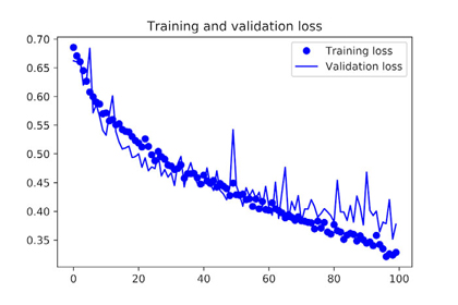
And let’s plot the results again: Thanks to data augmentation and dropout, you’re no longer overfitting: the training curves are closely tracking the validation curves. You now reach an accuracy of 82%, a 15% relative improvement over the non-regularized model.

• Training and validation accuracy with data augmentation

• Training and validation loss with data augmentation

By using regularization techniques even further, and by tuning the network’s parameters (such as the number of filters per convolution layer, or the number of layers in the network), you may be able to get an even better accuracy, likely up to 86% or 87%. But it would prove difficult to go any higher just by training your own convnet from scratch, because you have so little data to work with. As a next step to improve your accuracy on this problem, you’ll have to use a pretrained model, which is the focus of the next two sections.