8-4. Generating images with variational autoencoders

Sampling from a latent space of images to create entirely new images or edit existing ones is currently the most popular and successful application of creative AI. In this section and the next, we’ll review some high-level concepts pertaining to image generation, alongside implementation details relative to the two main techniques in this domain: variational autoencoders (VAEs) and generative adversarial networks (GANs). he techniques we present here aren’t specific to images—you could develop latent spaces of sound, music, or even text, using GANs and VAEs—but in practice, the most interesting results have been obtained with pictures, and that’s what we focus on here.

8.4.1 Sampling from latent spaces of images

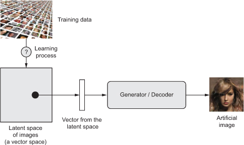
The key idea of image generation is to develop a low-dimensional latent space of representations (which naturally is a vector space) where any point can be mapped to a realistic-looking image. The module capable of realizing this mapping, taking as input a latent point and outputting an image (a grid of pixels), is called a generator (in the case of GANs) or a decoder (in the case of VAEs). Once such a latent space has been developed, you can sample points from it, either deliberately or at random, and, by mapping them to image space, generate images that have never been seen before

• Learning a latent vector space of images, and using it to sample new images

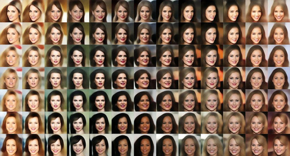
GANs and VAEs are two different strategies for learning such latent spaces of image representations, each with its own characteristics. VAEs are great for learning latent spaces that are well structured, where specific directions encode a meaningful axis of variation in the data. GANs generate images that can potentially be highly realistic, but the latent space they come from may not have as much structure and continuity.

• A continuous space of faces generated by Tom White using VAEs

8.4.2 Concept vectors for image editing

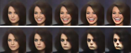
We already hinted at the idea of a concept vector when we covered word embeddings. The idea is still the same: given a latent space of representations, or an embedding space, certain directions in the space may encode interesting axes of variation in the original data. In a latent space of images of faces, for instance, there may be a smile vector, such that if latent point z is the embedded representation of a certain face, then latent point z + s is the embedded representation of the same face, smiling. Once you’ve identified such a vector, it then becomes possible to edit images by projecting them into the latent space, moving their representation in a meaningful way, and then decoding them back to image space. There are concept vectors for essentially any independent dimension of variation in image space— in the case of faces, you may discover vectors for adding sunglasses to a face, removing glasses, turning a male face into a female face, and so on. Below is an example of a smile vector, a concept vector discovered by Tom White from the Victoria University School of Design in New Zealand, using VAEs trained on a dataset of faces of celebrities (the CelebA dataset).

• The smile vector

8.4.3. Variational autoencoders

Variational autoencoders, simultaneously discovered by Kingma and Welling in December 2013 and Rezende, Mohamed, and Wierstra in January 2014, are a kind of generative model that’s especially appropriate for the task of image editing via concept vectors. They’re a modern take on autoencoders — a type of network that aims to encode an input to a low-dimensional latent space and then decode it back—that mixes ideas from deep learning with Bayesian inference.

Diederik P. Kingma and Max Welling, “Auto-Encoding Variational Bayes, arXiv (2013), https://arxiv.org/abs/1312.6114

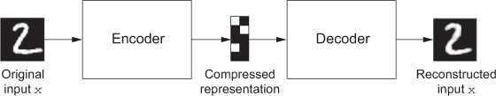
A classical image autoencoder takes an image, maps it to a latent vector space via an encoder module, and then decodes it back to an output with the same dimensions as the original image, via a decoder module. It’s then trained by using as target data the same images as the input images, meaning the autoencoder learns to reconstruct the original inputs. By imposing various constraints on the code (the output of the encoder), you can get the autoencoder to learn more-or-less interesting latent representations of the data. Most commonly, you’ll constrain the code to be low-dimensional and sparse (mostly zeros), in which case the encoder acts as a way to compress the input data into fewer bits of information.

• An autoencoder: mapping an input x to a compressed representation and then decoding it back as x'

In practice, such classical autoencoders don’t lead to particularly useful or nicely structured latent spaces. They’re not much good at compression, either. For these reasons, they have largely fallen out of fashion. VAEs, however, augment autoencoders with a little bit of statistical magic that forces them to learn continuous, highly structured latent spaces. . They have turned out to be a powerful tool for image generation.

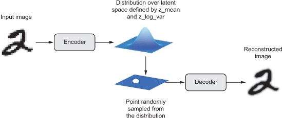
A VAE, instead of compressing its input image into a fixed code in the latent space, turns the image into the parameters of a statistical distribution: a mean and a variance. Essentially, this means you’re assuming the input image has been generated by a statistical process, and that the randomness of this process should be taken into account during encoding and decoding. The VAE then uses the mean and variance parameters to randomly sample one element of the distribution, and decodes that element back to the original input.

The stochasticity of this process improves robustness and forces the latent space to encode meaningful representations everywhere: every point sampled in the latent space is decoded to a valid output.

• A VAE maps an image to two vectors, z_mean and z_log_sigma, which define a probability distribution over the latent space, used to sample a latent point to decode.

In technical terms, here’s how a VAE works:

1. An encoder module turns the input samples input_img into two parameters in a latent space of representations, z_mean and z_log_variance.

2. You randomly sample a point z from the latent normal distribution that’s assumed to generate the input image, via z = z_mean + exp(z_log_variance) * epsilon, where epsilon is a random tensor of small values.

3. A decoder module maps this point in the latent space back to the original input image.

Because epsilon is random, the process ensures that every point that’s close to the latent location where you encoded input_img (z-mean) can be decoded to something similar to input_img, can be decoded to something similar to input_img, thus forcing the latent space to be continuously meaningful.

Any two close points in the latent space will decode to highly similar images. Continuity, combined with the low dimensionality of the latent space, forces every direction in the latent space to encode a meaningful axis of variation of the data, making the latent space very structured and thus highly suitable to manipulation via concept vectors.

The parameters of a VAE are trained via two loss functions:

1. reconstruction loss that forces the decoded samples to match the initial inputs,
2. regularization loss that helps learn well-formed latent spaces and reduce overfitting to the training data.

Let’s quickly go over a Keras implementation of a VAE. Schematically, it looks like this:

# Encodes the input into a mean and variance parameter
z_mean, z_log_variance = encoder(input_img)

# Draws a latent point using a small random epsilon
z = z_mean + exp(z_log_variance) * epsilon

# Decodes z back to an image
reconstructed_img = decoder(z)

# Instantiates the autoencoder model, which maps an input image to its reconstruction
model = Model(input_img, reconstructed_img)

You can then train the model using the reconstruction loss and the regularization loss.

The following listing shows the encoder network you’ll use, mapping images to the parameters of a probability distribution over the latent space. It’s a simple convnet that maps the input image x to two vectors, z_mean and z_log_var.

• VAE encoder network

import keras
from keras import layers
from keras import backend as K
from keras.models import Model
import numpy as np

img_shape = (28, 28, 1)
batch_size = 16
# Dimensionality of the latent space: a 2D plane
latent_dim = 2

input_img = keras.Input(shape=img_shape)

x = layers.Conv2D(32, 3,
                  padding='same', activation='relu')(input_img)
x = layers.Conv2D(64, 3,
                  padding='same', activation='relu',
                  strides=(2, 2))(x)
x = layers.Conv2D(64, 3,
                  padding='same', activation='relu')(x)
x = layers.Conv2D(64, 3,
                  padding='same', activation='relu')(x)
shape_before_flattening = K.int_shape(x)

x = layers.Flatten()(x)
x = layers.Dense(32, activation='relu')(x)

# The input image ends up being encoded into these two parameters.
z_mean = layers.Dense(latent_dim)(x)
z_log_var = layers.Dense(latent_dim)(x)

Next is the code for using z_mean and z_log_var, the parameters of the statistical distribution assumed to have produced input_img, to generate a latent space point z. Here, you wrap some arbitrary code (built on top of Keras backend primitives) into a Lambda layer. In Keras, everything needs to be a layer, so code that isn’t part of a built-in layer should be wrapped in a Lambda (or in a custom layer).

• Latent-space-sampling function

def sampling(args):
    z_mean, z_log_var = args
    epsilon = K.random_normal(shape=(K.shape(z_mean)[0], latent_dim),
                              mean=0., stddev=1.)
    return z_mean + K.exp(z_log_var) * epsilon

z = layers.Lambda(sampling)([z_mean, z_log_var])

The following listing shows the decoder implementation. You reshape the vector z to the dimensions of an image and then use a few convolution layers to obtain a final image output that has the same dimensions as the original input_img.

• VAE decoder network, mapping latent space points to images

# Input where you’ll feed z
decoder_input = layers.Input(K.int_shape(z)[1:])

# Upsamples the input
x = layers.Dense(np.prod(shape_before_flattening[1:]),
                 activation='relu')(decoder_input)

# Reshapes z into a feature map of the same shape as the feature map 
# just before the last Flatten layer in the encoder model
x = layers.Reshape(shape_before_flattening[1:])(x)

# Uses a Conv2DTranspose layer and Conv2D layer to decode z 
# into a feature map the same size as the original image input
x = layers.Conv2DTranspose(32, 3,
                           padding='same',
                           activation='relu',
                           strides=(2, 2))(x)
x = layers.Conv2D(1, 3,
                  padding='same',
                  activation='sigmoid')(x)

# Instantiates the decoder model, which turns “decoder_input” into the decoded image
decoder = Model(decoder_input, x)

# Applies it to z to recover the decoded z
z_decoded = decoder(z)