8-5. Introduction to generative adversarial networks

2018, Oct 01    

Generative adversarial networks (GANs), introduced in 2014 by Goodfellow et al., are an alternative to VAEs for learning latent spaces of images. They enable the generation of fairly realistic synthetic images by forcing the generated images to be statistically almost indistinguishable from real ones.

Ian Goodfellow et al., “Generative Adversarial Networks,” arXiv (2014)

An intuitive way to understand GANs is to imagine a forger trying to create a fake Picasso painting. At first, the forger is pretty bad at the task. He mixes some of his fakes with authentic Picassos and shows them all to an art dealer. The art dealer makes an authenticity assessment for each painting and gives the forger feedback about what makes a Picasso look like a Picasso. The forger goes back to his studio to prepare some new fakes. As times goes on, the forger becomes increasingly competent at imitating the style of Picasso, and the art dealer becomes increasingly expert at spotting fakes. In the end, they have on their hands some excellent fake Picassos.

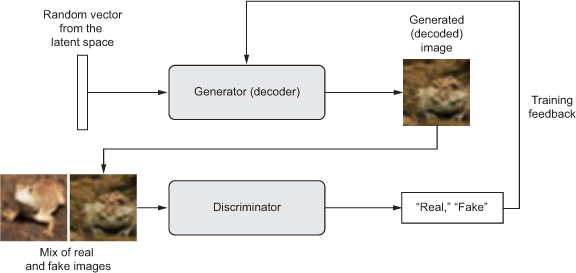
That’s what a GAN is: a forger network and an expert network, each being trained to best the other. As such, a GAN is made of two parts:

• Generator network - Takes as input a random vector (a random point in the latent space), and decodes it into a synthetic image
• Discriminator network(or adversary) - Takes as input an image (real or synthetic), and predicts whether the image came from the training set or was created by the generator network.

The generator network is trained to be able to fool the discriminator network, and thus it evolves toward generating increasingly realistic images as training goes on: artificial images that look indistinguishable from real ones, to the extent that it’s impossible for the discriminator network to tell the two apart Meanwhile, the discriminator is constantly adapting to the gradually improving capabilities of the generator, setting a high bar of realism for the generated images. Once training is over, the generator is capable of turning any point in its input space into a believable image. Unlike VAEs, this latent space has fewer explicit guarantees of meaningful structure; in particular, it isn’t continuous.

• A generator transforms random latent vectors into images, and a discriminator seeks to tell real images from generated ones. The generator is trained to fool the discriminator.

Remarkably, a GAN is a system where the optimization minimum isn’t fixed, unlike in any other training setup you’ve encountered. Normally, gradient descent consists of rolling down hills in a static loss landscape. But with a GAN, every step taken down the hill changes the entire landscape a little. It’s a dynamic system where the optimization process is seeking not a minimum, but an equilibrium between two forces. For this reason, GANs are notoriously difficult to train—getting a GAN to work requires lots of careful tuning of the model architecture and training parameters.

8.5.1. A schematic GAN implementation

In this section, we’ll explain how to implement a GAN in Keras. The specific implementation is a deep convolutional GAN (DCGAN): a GAN where the generator and discriminator are deep convnets. In particular, it uses a Conv2DTranspose layer for image upsampling in the generator.

You’ll train the GAN on images from CIFAR10, a dataset of 50,000 32 × 32 RGB images belonging to 10 classes (5,000 images per class). To make things easier, you’ll only use images belonging to the class “frog.”

Schematically, the GAN looks like this:

1. A generator network maps vectors of shape (latent_dim,) to images of shape (32, 32, 3).
2. A discriminator network maps images of shape (32, 32, 3) to a binary score estimating the probability that the image is real.
3. A gan network chains the generator and the discriminator together: gan(x) = discriminator(generator(x)). Thus this gan network maps latent space vectors to the discriminator’s assessment of the realism of these latent vectors as decoded by the generator.
4. You train the discriminator using examples of real and fake images along with “real”/“fake” labels, just as you train any regular image-classification model.
5. To train the generator, you use the gradients of the generator’s weights with regard to the loss of the gan model. This means, at every step, you move the weights of the generator in a direction that makes the discriminator more likely to classify as “real” the images decoded by the generator. In other words, you train the generator to fool the discriminator.

8.5.2. A bag of tricks

The process of training GANs and tuning GAN implementations is notoriously difficult. There are a number of known tricks you should keep in mind. Like most things in deep learning, it’s more alchemy than science: these tricks are heuristics, not theory-backed guidelines. They’re supported by a level of intuitive understanding of the phenomenon at hand, and they’re known to work well empirically, although not necessarily in every context.

Here are a few of the tricks used in the implementation of the GAN generator and discriminator in this section. It isn’t an exhaustive list of GAN-related tips; you’ll find many more across the GAN literature:

• We use tanh as the last activation in the generator, instead of sigmoid, which is more commonly found in other types of models.
• We sample points from the latent space using a normal distribution (Gaussian distribution), not a uniform distribution.
• Stochasticity is good to induce robustness. Because GAN training results in a dynamic equilibrium, GANs are likely to get stuck in all sorts of ways. Introducing randomness during training helps prevent this. We introduce randomness in two ways:
  • by using dropout in the discriminator
  • by adding random noise to the labels for the discriminator.
• Sparse gradients can hinder GAN training. In deep learning, sparsity is often a desirable property, but not in GANs. Two things can induce gradient sparsity:
  • Max pooling operation
    • Instead of max pooling, we recommend using strided convolutions for downsampling
  • ReLU activations
    • we recommend using a LeakyReLU layer instead of a ReLU activation. It’s similar to ReLU, but it relaxes sparsity constraints by allowing small negative activation values.
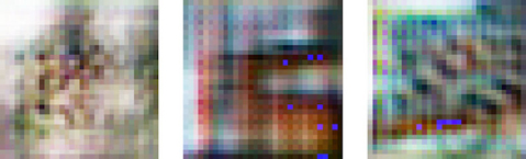
• In generated images, it’s common to see checkerboard artifacts caused by unequal coverage of the pixel space in the generator. To fix this, we use a kernel size that’s divisible by the stride size whenever we use a strided Conv2DTranpose or Conv2D in both the generator and the discriminator.

• Checkerboard artifacts caused by mismatching strides and kernel sizes, resulting in unequal pixel-space coverage: one of the many gotchas of GANs

8.5.3. The generator

First, let’s develop a generator model that turns a vector (from the latent space—during training it will be sampled at random) into a candidate image. One of the many issues that commonly arise with GANs is that the generator gets stuck with generated images that look like noise.

• A possible solution is to use dropout on both the discriminator and the generator.