What is Convolution Neural Network?
Introduction
In a regular neural network, the input is transformed through a series of hidden layers having multiple neurons.
Each neuron is connected to all the neurons in the previous and the following layers.
This arrangement is called a fully connected layer and the last layer is the output layer.
In Computer Vision applications where the input is an image, we use convolutional neural network because the regular fully connected neural networks don’t work well.
This is because if each pixel of the image is an input then as we add more layers the amount of parameters increases exponentially.
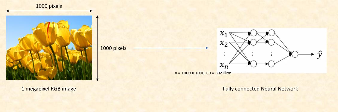
Consider an example where we are using a three color channel image with size 1 megapixel (1000 height X 1000 width) then our input will have 1000 X 1000 X 3 (3 Million) features. If we use a fully connected hidden layer with 1000 hidden units then the weight matrix will have 3 Billion (3 Million X 1000) parameters. So, the regular neural network is not scalable for image classification as processing such a large input is computationally very expensive and not feasible. The other challenge is that a large number of parameters can lead to over-fitting. However, when it comes to images, there seems to be little correlation between two closely situated individual pixels. This leads to the idea of convolution.
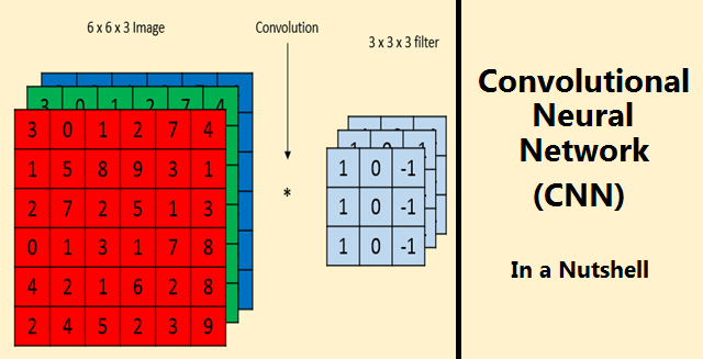
What is Convolution?
Convolution is a mathematical operation on two functions to produce a third function that expresses how the shape of one is modified by the other. The term convolution refers to both the result function and to the process of computing it. In a neural network, we will perform the convolution operation on the input image matrix to reduce its shape. In below example, we are convolving a 6 x 6 grayscale image with a 3 x 3 matrix called filter or kernel to produce a 4 x 4 matrix. First, we will take the dot product between the filter and the first 9 elements of the image matrix and fill the output matrix. Then we will slide the filter by one square over the image from left to right, from top to bottom and perform the same calculation. Finally, we will produce a two-dimensional activation map that gives the responses of that filter at every spatial position of input image matrix.
Challenges with Convolution
1. Shrinking output
One of the big challenges with convolving is that our image will continuously shrink if we perform convolutional operations in multiple layers. Let’s say if we have 100 hidden layers in our deep neural network and we perform convolution operation in every layer than our image size will shrink a little bit after each convolutional layer.
2. Data lost from the image corners
The second downside is that the pixels from the corner of the image will be used in few outputs only whereas the middle region pixels contribute more so we lose data from the corners of our original image. For example, the upper left corner pixel is involved in only one of the output but middle pixel contributed in at least 9 outputs.
Padding
In order to solve the problems of shrinking output and data lost from the image corners, we pad the image with additional borders of zeros called zero padding. The size of the zero padding is a hyperparameter. This allows us to control the spacial size of the output image. So if we define F as the size of our filter, S as the stride, N as the size of the image, and P as the amount of padding that we require, then the image output size is given by the following.
- Convolution on 6 x 6 image with zero padding = 1
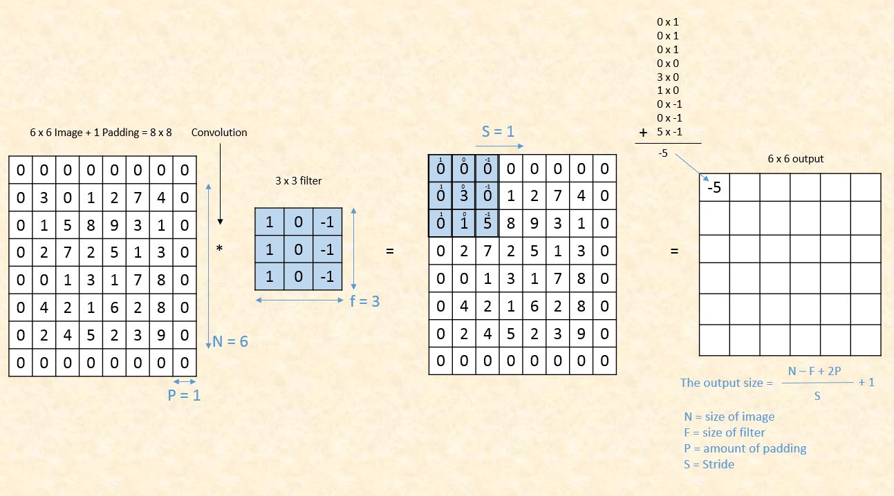
We can see that by using zero padding as 1, we have preserved the size of the original image. There are two common choices of padding. ‘Valid’ where we use P = 0 means no padding at all and ‘Same’ where the value of P is selected such that the size of the output image is equal to input image size. As far as filter size ‘F’ is concerned it is a recommended practice to select the odd number. Common choices are 1, 3, 5, 7…etc.
Convolution Over RGB Images
Earlier we saw the convolution operation on grey scale image (6 X 6). If our image is RGB then the dimensions will be 6 X 6 X 3 where 3 denotes the number of color channels. To detect the features in RGB images we use filters with 3 dimensions where the 3rd dimension will always be equal to the number of channels.
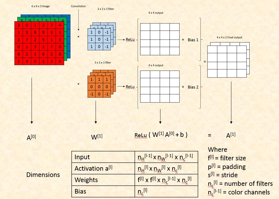
Single Layer of Convolutional Network
In one single layer of a convolutional network, we detect multiple features by convolving our image with different filters. Each convolution operation generates a different 2 dimensions matrix. We add bias to each of these matrices and then apply non-linearity. Then all of them were stacked together to form a 3-dimensional output. The third dimension of the final output will be equal to the number of filters used in convolution operation.
Dimensions of Convolutional Network
We will compare the convolution layer with regular neural network layer to calculate the number of parameters and dimensions.
- Dimension of Convolutional Layer Parameters
Pooling Layer
Though the total parameters of our network decrease after convolution still we need to further condense the spatial size of the representation to reduce the number of parameters and computation in the network. Pooling layer does this job for us and speeds up the computation as well as make some of the features more prominent. In pooling layer, we have two hyperparameters filter size and stride which are fixed only once. Following are two common types of pooling layers.
Max Pooling:
Let’s consider a 4 x 4 image matrix which we want to reduce to 2 x 2. We will use a 2 x 2 block with the stride size of 2. We will take the maximum value from each block and capture it in our new matrix.
Average Pooling:
In average pooling, we take the average of each of the blocks instead of the maximum value for each of the four squares.
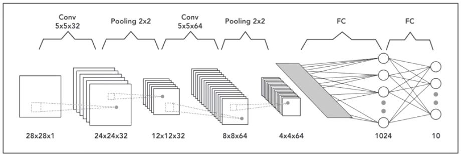
The Architecture of Convolutional Neural Network
A neural network that has one or multiple convolutional layers is called Convolutional Neural Network (CNN). Let’s consider an example of a deep convolutional neural network for image classification where the input image size is 28 x 28 x 1 (grayscale). In the first layer, we apply the convolution operation with 32 filters of 5 x 5 so our output will become 24 x 24 x 32. Then we will apply pooling with 2 x 2 filter to reduce the size to 12 x 12 x 32. In the second layer, we will apply the convolution operation with 64 filters of size 5 x 5. The output dimensions will become 8 x 8 x 64 on which we will apply pooling layer with 2 x 2 filter and the size will reduce to 4 x 4 x 64. Finally, we will pass it through two fully connected layers to convert our image matrix into a classification matrix.
Thank you for reading!!
Reference :
- https://en.wikipedia.org/wiki/Convolution
- Convolutional Neural Networks by Andrew Ng. (coursera.org)