Transformer 모델 (Attention is all you need)

deep learning 관련 글 목차

참조 : https://youtu.be/Yk1tV_cXMMU
참조 : https://youtu.be/xhY7m8QVKjo
참조 : https://charon.me/posts/pytorch/pytorch_seq2seq_6/
참조 : https://youtu.be/AA621UofTUA?list=RDCMUChflhu32f5EUHlY7_SetNWw
참조 : https://medium.com/@deepganteam/what-are-transformers-b687f2bcdf49
참조 : https://mlexplained.com/2017/12/29/attention-is-all-you-need-explained/
참조 : https://youtu.be/AA621UofTUA?list=RDCMUChflhu32f5EUHlY7_SetNWw
참조 : https://sanghyu.tistory.com/107
참조 : https://youtu.be/U0s0f995w14

Transformer의 특징

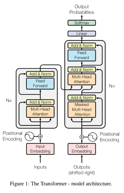
Transformer 모델의 구조는 위 그림과 같습니다. 이 모델은 번역 문제에서 RNN과 CNN을 쓰지 않고 Attention과 Fully Connected Layer와 같은 기본 연산만을 이용하여 SOTA 성능을 이끌어낸 연구로 유명합니다.
먼저 모델의 아키텍쳐에 대하여 간단히 살펴보겠습니다.
① Seq2seq와 유사한 Encoder - Decoder 형식을 사용합니다.
② Transformer에서 제안하는 Scaled Dot-Product Attention과 이를 병렬로 나열한 Multi-Head Attention 블록이 알고리즘의 핵심입니다.
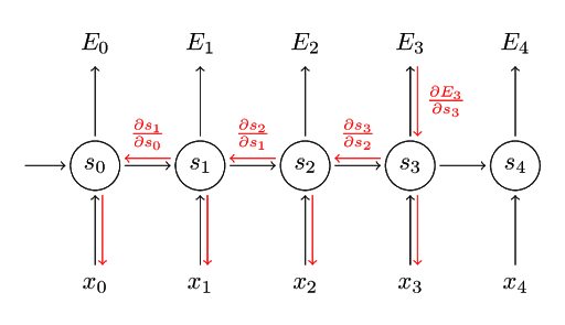
③ RNN의 구조에서는 아래 그림과 같은 BPTT (Back Propagation Through Time) 구조로 인하여 시간이 흐르는 기준으로 펼쳐놓고 봐야 하기 때문에 순차적인 연산이 필요합니다. 따라서 연산 효율이 떨어지는 문제가 발생합니다. Transformer 구조에서는 BPTT와 같은 구조가 없고 병렬 계산이 가능하기 때문에 RNN 구조에 비하여 굉장히 효율적으로 연산할 수 있습니다.

④ Transformer 같은 경우 RNN과 다르게 병렬적으로 계산할 수 있기 때문에 현재 계산하고 있는 단어가 어느 위치에 있는 단어인지를 표현을 해주어야 합니다. 그래서 Positional Encoding을 사용하고 있습니다.

Transformer와 Seq2seq의 차이점

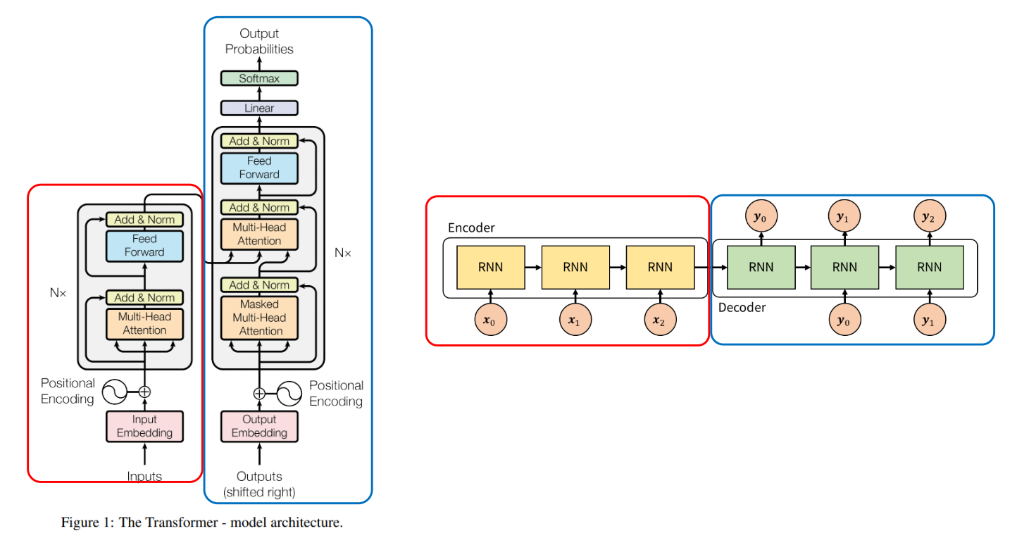
먼저 Transformer와 Seq2seq 비교를 통하여 구조를 알아보도록 하겠습니다.
Seq2seq의 경우 Encoder(빨간색)와 Decoder(파란색) 형태로 이루어져 있고 각 Encoder, Decoder에는 RNN을 사용하였습니다. 그리고 Encoder에서 Decoder로 정보를 전달할 때, 가운데 화살표인 context vector에 Encoder의 모든 정보를 저장하여 Decoder로 전달합니다.
반면 Transformer의 경우에도 Encoder(빨간색)와 Decoder(파란색) 형태가 있고 Encoder 끝단 부분에 Decoder로 전달되는 화살표가 있어서 Seq2seq와 유사한 구조를 가집니다.
하지만 가장 큰 차이점은 Seq2seq에서는 Encoder에 입력되어야 할 모든 인풋(ex. 단어)인 \(x_{0}, x_{1}, ...\)이 처리된 후에 Decoder 연산이 시작되나 Transformer에서는 Encoder의 계산과 Decoder의 계산이 동시에 일어나는 차이점이 있습니다.

Transformer의 입력과 출력

다음으로 Transformer의 입력과 출력의 형태에 대하여 알아보도록 하곘습니다.
Transformer 모델이 자연어 번역을 위해서 개발되었기 때문에 단어 벡터를 입출력 기준으로 설명하겠습니다.
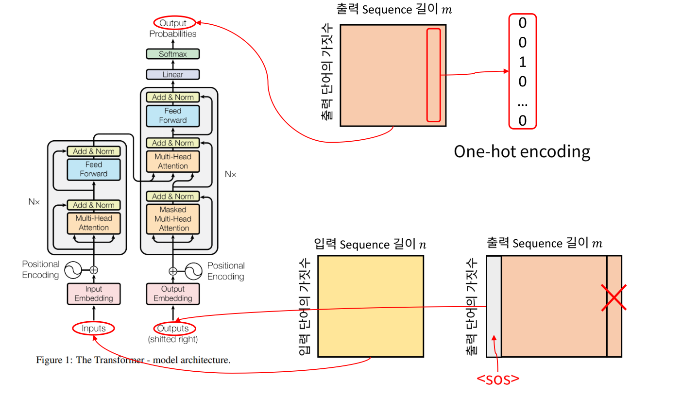
전체 입출력 형태를 보면 행렬과 같이 보입니다. 그러면 행렬의 행과 열은 무엇을 의미하는 지 살펴보겠습니다.

먼저 입력(Input)에 대하여 살펴보겠습니다.
각 단어는 One-hot Encoding 형태의 벡터로 나타내어 집니다. 따라서 열벡터가 한 단어에 해당하며 열 벡터의 길이 즉, 행렬에서 행의 크기는 입력 단어의 가짓수와 관련이 있습니다.
반면 열의 길이는 사용되는 sequence한 단어의 길이입니다. 문장에서 단어가 10개 있다면 행렬에서의 열의 크기는 10이 된다고 볼 수 있습니다.

다음은 출력(Output)에 대하여 살펴보겠습니다.
Transformer에서 처음 다룬 문제는 번역입니다. 따라서 출력도 단어 형태이나 입력과 출력의 행렬 사이즈는 다를 수 있습니다.
예를 들어 입력이 영어고 출력이 한국어이면 사용되는 단어의 갯수도 다를 뿐 아니라 같은 의미의 문장이라도 그 문장에서 사용되는 단어의 갯수도 다를 수 있기 때문입니다.
따라서 입력과 출력의 크기는 차이가 있을 수 있으나, 구성 성분은 동일합니다. 출력의 각 열 벡터의 크기 즉, 행렬의 행의 크기는 출력 단어의 가짓수와 관련이 있고 행렬의 열의 크기는 출력에서 사용되는 sequence한 단어의 길이를 나타냅니다.

입력과는 다르게 출력(Output)을 살펴보면 2가지의 Output이 표시되어 있습니다.
Seq2seq에서도 그림에서 위쪽에 있는 Output은 Transformer 모델을 통해 출력되는 실제 출력이고 아래쪽에 있는 Output은 Transformer에서 만들어낸 Output을 다시 입력으로 사용되는 것을 나타냅니다.
다시 입력되는 Output의 첫 열벡터는 SOS (Start Of Sequence)가 되고 X 표시가 되어있는 마지막 열벡터는 EOS (End Of Sequence)이므로 큰 의미는 없는 벡터입니다.
따라서 shifted right라고 적힌 부분은 Output 에서 하나씩 오른쪽으로 밀려서 다시 입력으로 들어가는 구조로 이해하시면 됩니다.

Transformer의 Word Embedding

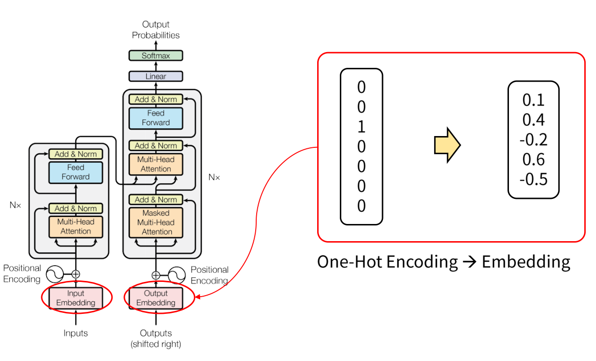
먼저 입력에 사용된 one-hot encoding 타입의 벡터를 실수 형태로 변경하면서 차원의 수를 줄일 수 있습니다.
위 그림과 같이 one-hot encoding 벡터를 실수 형태로 변경하면서 차원의 수를 줄일 수 있습니다.
Embedding의 경우 0을 기준으로 분포된 형태를 따르게 됩니다.

Positional Encoding

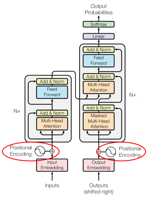
Word Embedding을 마치면 Positional Encoding을 통해 얻은 값과 Embedding이 더해지게 됩니다.
기존의 Seq2seq와는 다르게 Transformer에서는 입력 순서 대로 차례 차례 입력되지 않기 때문에 Positional Encoding을 통하여 시간적 위치 정보를 추가해 줍니다. 즉, 시간적 위치별로 고유의 Code를 생성하여 더하는 방식을 사용합니다.
따라서 전체 Sequence의 길이 중 상대적 위치에 따라 고유의 벡터를 생성하여 Embedding된 벡터에 더해줍니다.
Encoding은 sin, cos 함수를 통하여 생성된 값으로 이 주기 함수에 대한 규칙을 모델이 학습을 통하여 배움으로써 입력 값의 상대적 위치를 알 수 있게 됩니다.

\[\text{PE}_{(\text{pos}, 2i)} = \sin{(\text{pos}/10000^{2i / \text{d}_{\text{model}}})}\]
\[\text{PE}_{(\text{pos}, 2i+ 1)} = \cos{(\text{pos}/10000^{2i / \text{d}_{\text{model}}})}\]

pos는 상대적 위치를 뜻하고 i는 벡터의 인덱스를 뜻합니다.
최근에는 기존의 Transformer에서 제시하는 sin, cos 방식 보다는 nn.Embedding(max_length, embed_size)와 같은 embedding 방식을 이용하여 학습하는 방식을 많이 사용하고 있습니다. 이 방식이 더 좋은 성능을 내서 Transformer를 활용하는 BERT, GPT 등에도 Embedding을 이용한 학습 기법을 사용합니다.

self.tok_embedding = nn.Embedding(input_dim, hidden_dim)
# positional encoding
self.pos_embedding = nn.Embedding(max_length, hidden_dim)

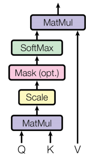
Scaled Dot-Product Attention

이 글의 처음 도입부에서 설명하였듯이 Transformer의 핵심이 되는 것이 Scaled Dot-Product Attention이라고 하였습니다.
먼저 Attention 내용이 정확히 기억이 나지 않으시면 아래 링크를 참조하시기 바랍니다.
- 링크 : https://gaussian37.github.io/dl-concept-attention/

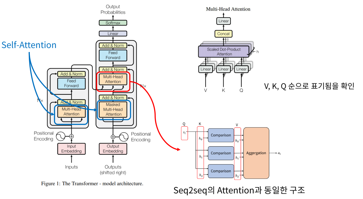
Attention에서 사용되는 입력은 Q(Query), K(Key), V(Value) 입니다. 따라서 Scaled Dot-Product Attention 에서도 Query, Key, Value 구조를 띕니다.
Q와 K의 비교 함수는 Dot-Product와 Scale로 이루어 집니다. Dot-Product는 위 그림에서 MatMul에 해당하고 간단히 inner product (내적)과 같습니다.
그리고 Mask를 이용해 illegal connection의 attention을 금지합니다. illegal connection은 self-attention 개념과 연관되어 있습니다.
self-attention은 각각의 입력이 서로 다른 입력에게 어떤 연관성을 가지고 있는 지를 구하기 위해 사용됩니다.

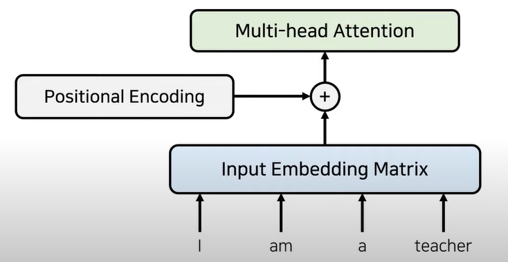
예를 들어 self-attention은 입력 문장에 대하여 문맥에 대한 정보를 잘 학습하도록 만들 수 있습니다. 즉, “I am a teacher”에서 각 단어가 서로 어떤 연관성을 가지고 있는 지 학습할 수 있습니다.
그러면 self-attention 개념과 연관된 illegal connection에 대하여 간략하게 알아보겠습니다.

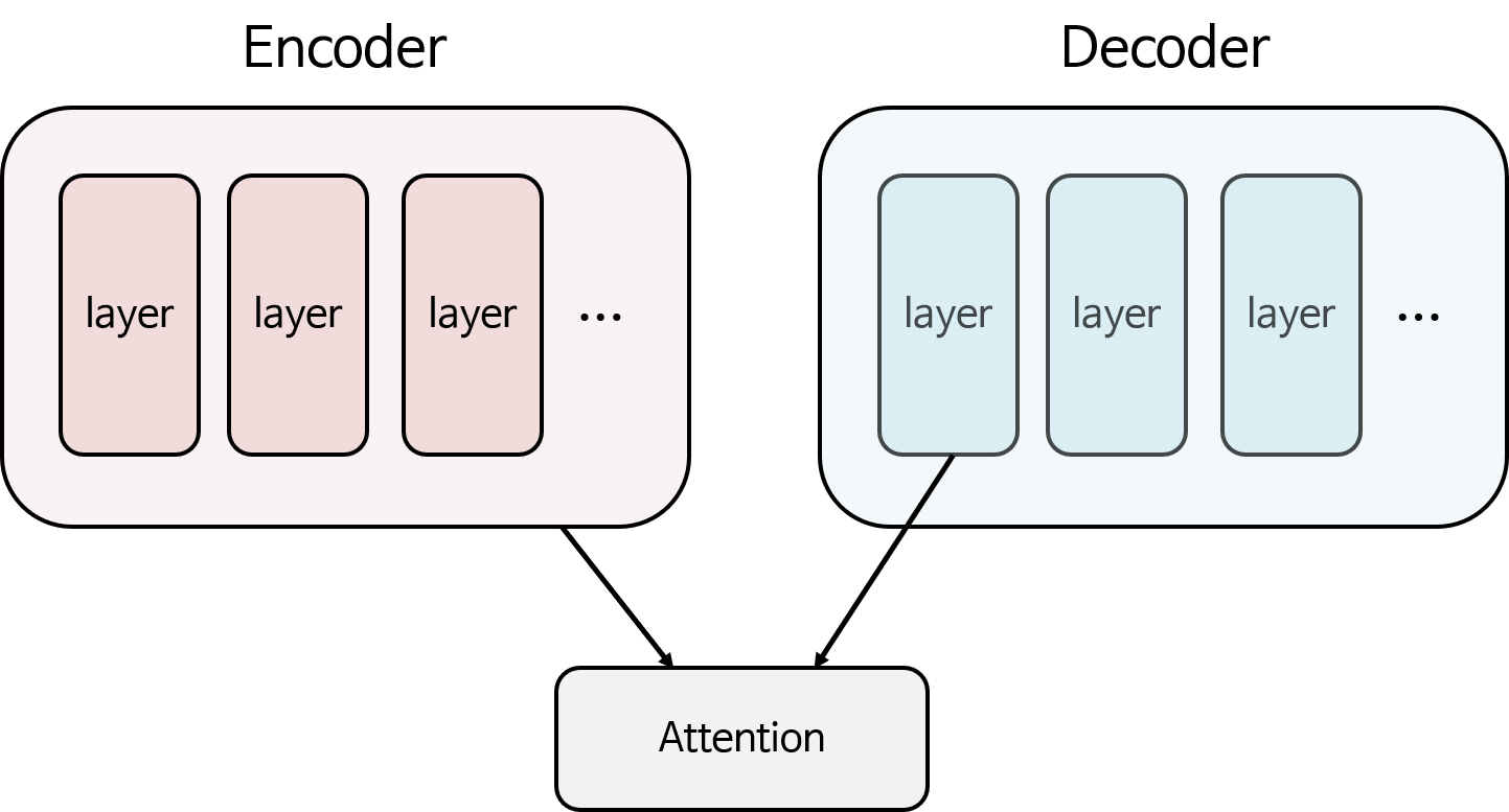
Seq2seq에서 사용된 Attention 메커니즘을 살펴보면 Encoder에서 사용된 모든 Step 별 layer와 Decoder의 특정 layer를 이용하여 Attention 연산을 하였습니다. 따라서 위 그림과 같이 Encoder에서 사용된 전체 layer와 Decoder에서는 첫번째, 두번째, … 차례대로 Attention 연산을 하여 Decoder의 어떤 layer가 Encoder의 어떤 layer에 매칭되는 지 알 수 있습니다.

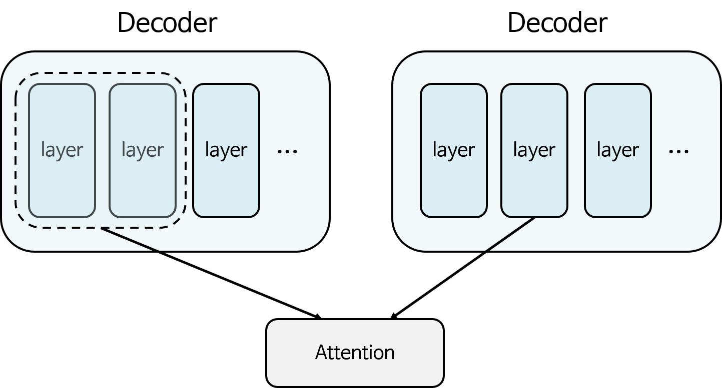
self-attention에서는 Decoder가 똑같은 Decoder 자신과 Attention 연산을 할 수 있습니다. 위 그림과 같이 오른쪽의 2번째 layer의 Attention 연산을 하기 위해서는 Decoder의 전체 layer를 사용할 수 없습니다. 왜냐하면 Decoder에서 순차적으로 출력이 나온다고 생각하였을 때, 아직 3번째 layer 부터는 출력이 나오지 않았기 때문입니다. 따라서 1, 2번째 layer만 Attention 연산이 가능합니다.
따라서 self-attention을 하기 위해서는 어느 특정 layer 보다 앞선 layer 들만 가지고 Attention을 할 수 있습니다.
그러면 illegal connection은 2번째 layer를 대상으로 self-Attention 연산 시 3번째, 4번째 layer들도 같이 Attention에 참여되는 상황입니다. 즉, 미래에 출력되는 output을 가져다 쓴것인데 이런 문제를 방지해야 합니다.
이 내용을 현재 Transformer에 접목해 보겠습니다.

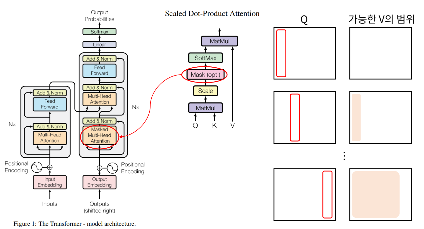
위 그림에서 오른쪽 Q와 가능한 V의 범위를 살펴보면 선택된 Q에 대하여 가능한 V의 범위는 위치상 Q의 바로 앞까지임을 알 수 있습니다.
따라서 mask를 이용하여 이러한 illegal connection의 attention을 금지해줍니다.
정리하면 Self-Attention에서는 자기 자신을 포함한 미래의 값과는 Attention을 구하지 않기 때문에 Masking을 사용합니다.
mask에 해당되는 값은 음의 무한대로 값을 변경해 버리면 그 다음 스텝의 SoftMax에서 0이 되기 때문에 무시해 버릴 수 있습니다.
최종적으로 SoftMax의 출력인 유사도와 V를 결합하여 Attention Value를 계산합니다.

이 때, Q, K, V 각각은 다음과 같이 행렬 형태로 변환 후 연산됩니다.

\[Q = [q_{0}, q_{1}, \cdots , q_{n}]\]
\[K = [k_{0}, k_{1}, \cdots , k_{n}]\]
\[V = [v_{0}, v_{1}, \cdots , v_{n}]\]

이와 같이 행렬 형태로 변환하는 이유는 병렬 연산을 하기 위함입니다.

\[C = \text{softmax} \Biggl(\frac{K^{T}Q}{\sqrt{d_{k}}}\Biggr)\]

위 식의 \(C\)는 Scaled Dot-Product Attention의 softmax 까지의 결과 입니다.
먼저 \(K^{T}Q\)를 통하여 Key와 Query를 Dot-Product 형태로 연산을 하고 \(\sqrt{d_{k}}\)를 통하여 Scale을 해줍니다. 이 Scale 값을 통해 \(K^{T}Q\) 값이 너무 커지거나 작아져서 softmax의 결과가 0에 가깝게 saturation이 되는 것을 방지합니다.

그 다음 \(C\) 값과 \(V\)값을 \(C^{T} V = \text{softmax} \Biggl(\frac{K^{T}Q}{\sqrt{d_{k}}}\Biggr)V = a\) 와 같이 연산을 하여 Attention Value \(a\)를 구할 수 있습니다.
위 식들을 살펴보면 행렬의 곱과 softmax의 형태로만 이루어져 있습니다. 행렬의 곱은 GPU를 이용하여 병렬 연산 처리가 가능하기 때문에 연산 속도가 빨라집니다. 이 점이 Transformer의 가장 큰 장점 중 하나라고 말할 수 있습니다.

Multi-Head Attention

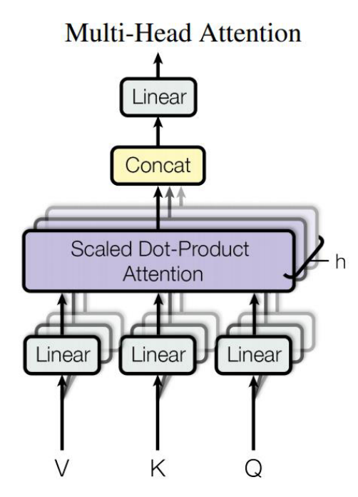
Multi-Head Attention은 Scaled Dot-Product Attention을 h개 모아서 Attention Layer를 병렬적으로 사용하는 것을 말합니다.
즉, 한번에 전체 Scaled Dot-Product Attention을 연산하기 보다 여러 개의 작은 Scaled Dot-Product Attention으로 분할하고 병렬적으로 연산한 다음에 다시 concat하여 합치는 divide & conquer 전략이라고 생각할 수 있습니다.
따라서 Scaled Dot-Product Attention에서 몇개(h개)로 분할하여 연산할 지에 따라서 각각의 Scaled Dot-Product Attention의 입력 크기가 달라지게 됩니다.
정리하면 Linear 연산 (Matrix Multiplication)을 이용해 Q, K, V의 차원을 감소하고 Q와 K의 차원이 다를 경우 이를 이용해 동일한 차원으로 맞춰서 Scaled Dot-Product Attention을 위한 입력으로 만들어 줍니다. 차원이 어떻게 변화하는 지 아래 수식으로 살펴보겠습니다.

\[\text{Linear}_{i}(V) = V W_{V, i} \ \ \ \ W_{V, i} \in \mathbb{R}^{d_{V} \times d_{\text{model}}}\]
\[\text{Linear}_{i}(K) = K W_{K, i} \ \ \ \ W_{K, i} \in \mathbb{R}^{d_{K} \times d_{\text{model}}}\]
\[\text{Linear}_{i}(Q) = Q W_{Q, i} \ \ \ \ W_{Q, i} \in \mathbb{R}^{d_{Q} \times d_{\text{model}}}\]

위 수식에서 \(W\)는 차원을 변경하기 위한 행렬 입니다. \(d_{v}, d_{k}, d_{q}\) 각각은 Value, Key, Query의 dimension을 뜻하고 \(d_{\text{model}}\)은 Multi-head Attention에서 Scaled Dot-Product Attention에 사용되는 dimension을 뜻합니다.

Linear 연산을 통해 Q, K, V의 차원을 감소하는 것은 모델이 어느 특정한 차원들만 선택해서 보겠다는 것을 의미합니다. h개의 방법으로 차원을 축소해서 보되 병렬적으로 전체를 검토하게 되므로 병렬 연산으로 연산 속도는 증가 시키면서 다방면으로 모델이 학습할 수 있도록 합니다.
위 그림과 같이 h개의 Scaled Dot-Product Attention은 병렬적이지만 독립되어 있습니다. h개 모듈을 병렬적으로 계산한 다음 concat 후 출력을 내주게 됩니다.
concat을 하게 되면 채널이 커질 수 있기 때문에 출력 직전 Linear 연산을 이용해 Attention Value의 차원을 필요에 따라 변경할 수 있습니다.
이와 같은 메커니즘을 통해 병렬 계산에 유리한 구조를 만들 수 있습니다.

Transformer 전체 구조에서 Multi-Head Attention이 어떻게 사용되는 지 살펴보겠습니다.
파란색으로 표시된 부분은 Self-Attention 구조로 들어가 있습니다. Self-Attention에서는 Key, Value, Query가 모두 같음을 의미합니다. Encoder의 파란색 부분은 Mask 없이 Key, Value, Query가 들어가게 됩니다. 반면 Decoder의 파란색 부분은 Mask가 적용됩니다. 왜냐하면 Key와 Value가 Query 하고자 하는것 보다 더 앞서서 등장할 수 없기 때문입니다. 이와 같이 Self-Attention을 통해서 Attention이 강조되어 있는 feature를 추출할 수 있습니다.
빨간색으로 표시된 Multi-Head Attention은 Encoder로 부터 Key와 Value를 받고 Decoder로 부터 Query를 받습니다. 이를 통해 Seq2seq의 Attention과 동일한 구조를 가지게 됩니다.

class MultiHeadAttentionLayer(nn.Module):
    # hidden_dim : embedding dimension of word
    # n_head : number of heads
    def __init__(self, hidden_dim, n_heads, dropout_ratio, device):
        super().__init__()
        
        assert(hidden_dim % n_heads == 0), "hidden_dim size needs to be div by n_heads"
        
        # embedding dimension
        self.hidden_dim = hidden_dim 
        # the number of heads : Number of different attention concepts
        self.n_heads = n_heads
        # Embedding dimension at each head
        self.head_dim = hidden_dim // n_heads

        # Basically, dimension is converted from hidden_dim to the key dimension.
        # Since the dimension of the key is hidden_dim, it is converted from hidden_dim to hidden_dim.
        ## FC layer to be applied to query
        self.fc_q = nn.Linear(hidden_dim, hidden_dim) 
        ## FC layer to be applied to key
        self.fc_k = nn.Linear(hidden_dim, hidden_dim)
        ## FC layer to be applied to value
        self.fc_v = nn.Linear(hidden_dim, hidden_dim)
        
        self.fc_o = nn.Linear(hidden_dim, hidden_dim)
        
        self.dropout = nn.Dropout(dropout_ratio)
        self.scale = torch.sqrt(torch.FloatTensor([self.head_dim])).to(device)

    def forward(self, query, key, value, mask=None):
        
        batch_size = query.shape[0]
        
        # query : [batch_size, query_len, hidden_dim] → Q : [batch_size, query_len, hidden_dim]
        Q = self.fc_q(query)
        # key : [batch_size, key_len, hidden_dim] → K : [batch_size, key_len, hidden_dim]
        K = self.fc_k(key)
        # value : [batch_size, value_len, hidden_dim] → V : [batch_size, value_len, hidden_dim]
        V = self.fc_v(value)
        
        # Seperate hidde_dim to n_heads*head_dim
        # Learn n_heads kinds of different attention concepts.
        
        # Q : [batch_size, query_len, hidden_dim]
        ## → Q : [batch_size, query_len, n_heads, head_dim]
        ### → Q : [batch_size, n_heads, query_len, head_dim]
        Q = Q.reshape(bath_size, -1, self.n_heads, self.head_dim).permute(0, 2, 1, 3)
        
        # K : [batch_size, key_len, hidden_dim]
        ## → K : [batch_size, key_len, n_heads, head_dim]
        ### → K : [batch_size, n_heads, key_len, head_dim]
        K = K.reshape(bath_size, -1, self.n_heads, self.head_dim).permute(0, 2, 1, 3)
        
        # V : [batch_size, value_len, hidden_dim]
        ## → V : [batch_size, value_len, n_heads, head_dim]
        ### → V : [batch_size, n_heads, value_len, head_dim]
        V = V.reshape(bath_size, -1, self.n_heads, self.head_dim).permute(0, 2, 1, 3)
        
        # Calculate attention energe
        # Q : [batch_size, n_heads, query_len, head_dim]
        # K.permute : [batch_size, n_heads, head_dim, key_len]
        
        # energy : [batch_size, n_heads, query_len, key_len]
        energy = torch.matmul(Q, K.permute(0, 1, 3, 2)) / self.scale
        
        if mask != None:
            # Fill in the part where the mask value is 0 with a very small value.
            energy = energy.masked_fill(mask==0, -1e10)
        
        # calculate attention score : probability about each data(ex.word)
        # We get attention score based on key_len.
        # attention : [batch_size, n_heads, query_len, key_len]
        attention = torch.softmax(energy, dim=-1)
        
        # attention : [batch_size, n_heads, query_len, key_len]
        # V : [batch_size, n_heads, value_len, head_dim]
        # x : [batch_size, n_heads, query_len, head_dim] (∵ key_len = value_len in this self-attention)
        x = torch.matmul(self.dropout(attention), V)
        
        # x : [batch_size, n_heads, query_len, head_dim]
        # → x : [batch_size, query_len, n_heads, head_dim]
        x = x.permute(0, 2, 1, 3).contiguous()
        
        # x : [batch_size, query_len, hidden_dim]
        x = x.reshape(batch_size, -1, self.hidden_dim)
        
        # x : [batch_size, query_len, hidden_dim]
        x = self.fc_o(x)
        
        return x, attention

Position-wise Feed-Forward

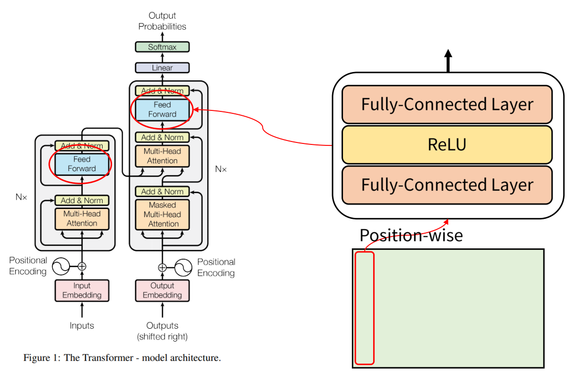
Position wise Feed Forward는 단어의 Position 별로 Feed Forward 한다는 뜻입니다. 각 단어에 해당하는 열 벡터가 입력으로 들어갔을 때, FC-layer - Relu - Fc-layer 연산을 거치게 됩니다.

class PositionwiseFeedForwardLayer(nn.Module):
    # hidden_dim : embedding dimension of a word
    # pf_dim : inner embedding dimension in feed forward layer
    # dropout_ratio
    def __init__(self, hidden_dim, pf_dim, dropout_ratio):
        super().__init__()
        
        self.fc_1 = nn.Linear(hidden_dim, pf_dim)
        self.fc_2 = nn.Linear(pf_dim, hidden_dim)
        
        self.dropout = nn.Dropout(dropout_ratio)
        
    def forward(self, x):
        # x : [batch_size, seq_len, hidden_dim]
        # → x : [batch_size, seq_len, pf_dim]
        x = self.dropout(torch.relu(self.fc_1(x)))
        # → x : [batch_size, seq_len, hidden_dim]
        x = self.fc_2(x)
        
        return x

Add & Norm

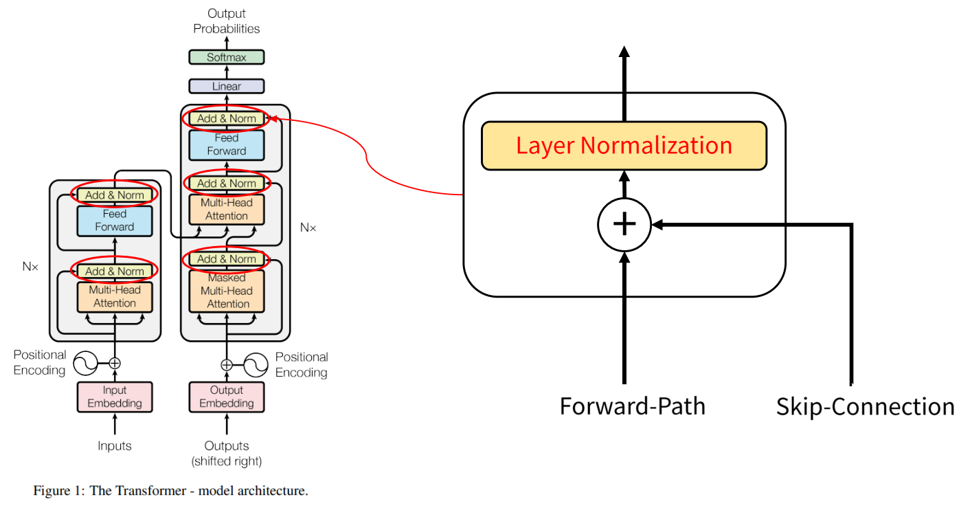
Transformer 구조를 보면 Skip Connection을 통해서 합해지는 부분이 있고 더해지는 부분에서 Layer Normalization을 사용하였습니다.
Layer Normalization에 대한 설명은 다음 링크를 참조하시기 바랍니다.
- 링크 :

Encoder Decoder 구조

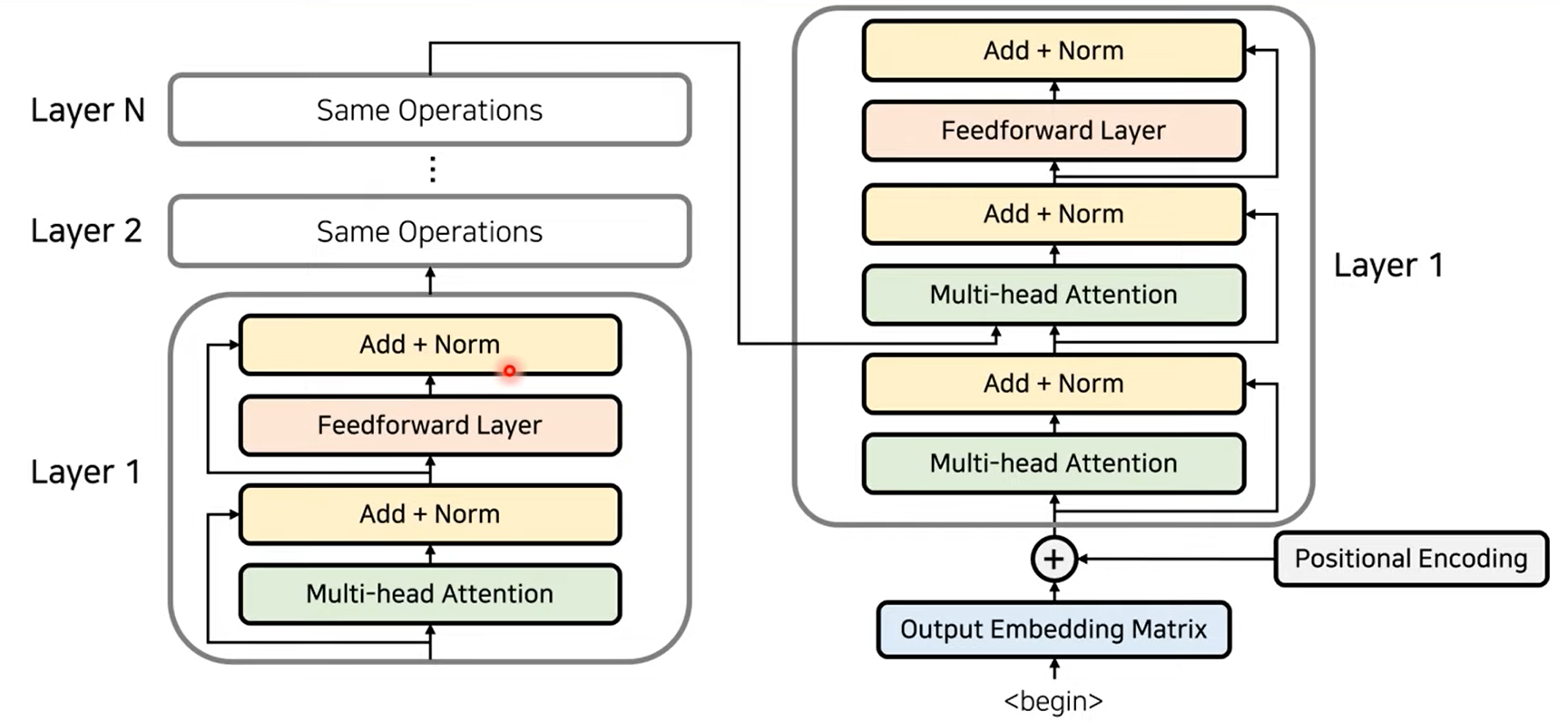
앞에서 설명한 Encoder와 Decoder의 구조를 간략이 나타내면 위 그림과 같습니다.
Encoder의 Input과 Output의 크기는 같습니다. 따라서 Encoder의 구조를 여러번 반복해서 사용하기 용이합니다.
위 그림과 같이 Encoder 부분을 여러번 반복하여 사용할 수 있습니다. Decoder 또한 여러번 반복하여 사용할 수 있습니다.

먼저 Encoder 구조는 다음과 같습니다.

class EncoderLayer(nn.Module):
    # Dimension of input and output are same.
    # Encoder of transformer uses multiple times encoder layer by using characteristics above.
    # set mask value 0 to <pad> token
    
    # hidden_dim : embedding dimension of a word
    # n_heads : the number of heads = the number of scaled-dot product attention
    # pf_dim : inner embedding dimension in feed-forward layer
    # dropout_ratio : dropout ratio
    def __init__(self, hidden_dim, n_heads, pf_dim, dropout_ratio, device):
        super().__init__()
        
        self.self_attention_layer_norm = nn.LayerNorm(hidden_dim)
        self.feedforward_layer_norm = nn.LayerNorm(hidden_dim)
        self.self_attention = MultiHeadAttentionLayer(hidden_dim, n_heads, dropout_ratio, device)
        self.potisionwise_feedforward = PositionwiseFeedForwardLayer(hidden_dim, pf_dim, dropout_ratio)
        self.dropout = nn.Dropout(dropout_ratio) 
        
    def forward(self, src, src_mask):
        # src : [batch_size, src_len, hidden_dim]
        # src_mask : [batch_size, src_len]
        
        # self attention
        # you can regulate words to apply attention with mask matrix.
        # _src : [batch_size, src_len, hidden_dim]
        _src, _ = self.self_attention(src, src, src, src_mask)
        
        # dropout, residual connection, layer normalization
        # src : [batch_size, src_len, hidden_dim]
        # _src : [batch_size, src_len, hidden_dim]
        # → src : [batch_size, src_len, hidden_dim]
        src = self.self_attention_layer_norm(src + self.dropout(_src))
        
        # position-wise feedforward 
        # src : [batch_size, src_len, hidden_dim]
        # _src : [batch_size, src_len, hidden_dim]
        _src = self.potisionwise_feedforward(src)
        
        # dropout, residual connection, layer normalization
        # src : [batch_size, src_len, hidden_dim]
        # _src : [batch_size, src_len, hidden_dim]
        # → src : [batch_size, src_len, hidden_dim]
        src = self.feedforward_layer_norm(src + self.dropout(_src))
        
        return src


class Encoder(nn.Module):
    
    # set mask value 0 to <pad> token. (<pad> token filled up after <eos>)
    # implemented positional encoding with nn.Embedding not sin, cos function. 

    # input_dim : one hot encoding dimension of a word
    # hidden_dim : embedding dimension of input_dim
    # n_layers : the number of encoder layer
    # n_heads : the number of heads = the number of scaled-dot product attention
    # pf_dim : inner embedding dimension in feed-forward layer
    # dropout_ratio : dropout ratio
    # max_length : maximum number of words in sentence
    
    def __init__(self, input_dim, hidden_dim, n_layers, n_heads, pf_dim, dropout_ratio, device, max_length=100):
        super().__init__()
        
        self.device = device
        # input dimenstion → embedding dimension
        self.tok_embedding = nn.Embedding(input_dim, hidden_dim)
        # positional encoding
        self.pos_embedding = nn.Embedding(max_length, hidden_dim)
        
        self.layers = nn.ModuleList([EncoderLayer(hidden_dim, n_heads, pf_dim, dropout_ratio, device) for _ in range(n_layers)])
        
        self.dropout = nn.Dropout(dropout_ratio)
        
        self.scale = torch.sqrt(torch.FloatTensor([hidden_dim])).to(device)
        
    def forward(self, src, src_mask):
        
        # src : [batch_size, src_len]
        # src_mask : [batch_size, src_len]
        
        # batch_size : the number of sentence
        batch_size = src.shape[0]
        # src_len : The number of words in the sentence with the maximum number of words among all sentences
        src_len = src.shape[1]
        
        # pos : [batch_size, src_len]
        pos = torch.arange(0, src_len).repeat(batch_size, 1).to(self.device)
        
        # use addition tensor of src embedding and pos embedding
        # src : [batch_size, src_len]
        # → src : [batch_size, src_len, hidden_dim]
        src = self.dropout((self.tok_embedding(src) * self.scale) + self.pos_embedding(pos))
        
        # Feed Forward through all encoder layer sequentially
        # src : [batch_size, src_len, hidden_dim]
        for layer in self.layers:
            src = layer(src, src_mask)
        
        return src

다음으로 Decoder 구조는 다음과 같습니다.

class DecoderLayer(nn.Module):
    # Dimension of input and output are same.
    # Decoder of transformer uses multiple times encoder layer by using characteristics above.
    # Decoder layer use two multi-head attention layer
    # set mask value 0 to <pad> token
    # Each word in the target sentence uses a mask to make it impossible to know what the next word is (see only the previous word).
    
    # hidden_dim : embedding dimension of input_dim
    # n_heads : the number of heads = the number of scaled-dot product attention
    # pf_dim : inner embedding dimension in feed-forward layer
    # dropout_ratio : dropout ratio
    
    def __init__(self, hidden_dim, n_heads, pf_dim, dropout_ratio, device):
        super().__init__()
        
        self.self_attention_layer_norm = nn.LayerNorm(hidden_dim)
        self.encoder_attention_layer_norm = nn.LayerNorm(hidden_dim)
        self.feedforward_layer_norm = nn.LayerNorm(hidden_dim)
        self.self_attention = MultiHeadAttentionLayer(hidden_dim, n_heads, dropout_ratio, device)
        self.encoder_attention = MultiHeadAttentionLayer(hidden_dim, n_heads, dropout_ratio, device)
        self.potisionwise_feedforward = PositionwiseFeedForwardLayer(hidden_dim, pf_dim, dropout_ratio)
        self.dropout = nn.Dropout(dropout_ratio) 
        
    # applied attention to encoder output (encoder_src)
    def forward(self, trg, encoder_src, trg_mask, src_mask):
        
        # trg : [batch_size, trg_len, hidden_dim]
        # encoder_src : [batch_size, src_len, hidden_dim]
        # trg_mask : [batch_size, trg_len]
        # src_mask : [batch_size, src_len]
        
        # self-attention
        # _trg : [batch_size, trg_len, hidden_dim]
        _trg, _ = self.self_attention(trg, trg, trg, trg_mask)
        
        # dropout, residual connection and layer normalization
        # trg : [batch_size, trg_len, hidden_dim]
        trg = self.self_attention_layer_norm(trg + self.dropout(_trg))
        
        # encoder attention
        # applied encoder attention by using decoder query
        _trg, attention = self.encoder_attention(trg, encoder_src, encoder_src, src_mask)
        
        # dropout, residual connection and layer normalization
        trg = self.encoder_attention_layer_norm(trg + self.dropout(_trg))
        
        # positionwise feedforward
        _trg = self.potisionwise_feedforward(trg)
        
        # dropout, residual and layer normalization
        trg = self.feedforward_layer_norm(trg + self.dropout(_trg))
        
        # trg : [batch_size, trg_len, hidden_dim]
        # attention : [batch_size, n_heads, trg_len, src_len]
        
        return trg, attention

class Decoder(nn.Module):
    
    # set mask value 0 to <pad> token. (<pad> token filled up after <eos>)
    # implemented positional encoding with nn.Embedding not sin, cos function. 
    
    # output_dim : one-hot encoding dimension of a word
    # hidden_dim : embedding dimension of a word
    # n_layers : the number of encoding layers
    # n_heads : the number of heads = the number of scaled-dot product attention
    # pf_dim : inner embedding dimension in feed-forward layer
    # dropout_ratio : dropout ratio
    # max_length : maximum number of words in sentence
    
    # set mask value 0 to <pad> token
    # Each word in the target sentence uses a mask to make it impossible to know what the next word is (see only the previous word).
    
    def __init__(self, output_dim, hidden_dim, n_layers, n_heads, pf_dim, dropout_ratio, device, max_length):
        super().__init__()
        
        self.device = device
        
        self.tok_embedding = nn.Embedding(output_dim, hidden_dim)
        self.pos_embedding = nn.Embedding(max_length, hidden_dim)
        
        self.layers = nn.ModuleList([DecoderLayer(hidden_dim, n_heads, pf_dim, dropout_ratio, device) for _ in range(n_layers)])
        
        self.fc_out = nn.Linear(hidden_dim, output_dim)
        
        self.dropout = nn.Dropout(dropout_ratio)
        
        self.scale = torch.sqrt(torch.FloatTensor([hidden_dim])).to(device)
        
    def forward(self, trg, encoder_src, trg_mask, src_mask):
        
        # trg : [batch_size, trg_len]
        # encoder_src : [batch_size, src_len, hidden_dim]
        # trg_mask : [batch_size, trg_len]
        # src_mask : [batch_size, src_len]
        
        batch_size = trg.shape[0]
        trg_len = trg.shape[1]
        
        # pos : [batch_size, trg_len]
        pos = torch.arange(0, trg_len).repeat(batch_size, 1).to(self.device)
        
        # trg : [batch_size, trg_len, hidden_dim]
        # attention : [batch_size, n_heads, trg_len, src_len]
        for layer in self.layers:
            trg, attention = layer(trg, encoder_src, trg_mask, src_mask)
            
        # output : [batch_size, trg_len, output_dim]
        output = self.fc_out(trg)
        
        return output, attention

Output Softmax

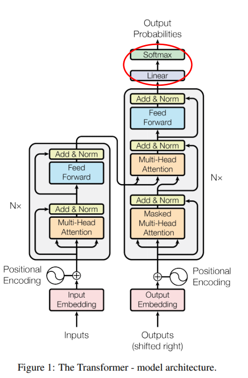
마지막 Feed Forward를 통해 출력이 되면 Linear 연산을 통하여 출력 단어 종류 갯수로 출력 사이즈를 맞춰 줍니다.
최종적으로 Softmax를 이용해 어떤 단어인지 Classification 문제를 해결할 수 있습니다.

class Transformer(nn.Module):
    def __init__(self, encoder, decoder, src_pad_idx, trg_pad_idx, device):
        super.__init__()
        
        self.encoder = encoder
        self.decoder = decoder
        self.src_pad_idx = src_pad_idx
        self.trg_pad_idx = trg_pad_idx
        self.device = device
        
    # set mask value as zero to <pad> token of src
    def make_src_mask(self, src):
        
        # src : [batch_size, src_len]
        src_mask = (src != self.src_pad_idx).unsqueeze(1).unsqueeze(2)
        
        # src_mask : [batch_size, 1, 1, src_len]
        return src_mask
    
    # Each word in the target word uses a mask to make it impossible to know what the next word is (see only the previous word).
    def make_trg_mask(self, trg):
        
        # trg : [batch_size, trg_len]
        
        '''
        mask example
        1 0 0 0 0
        1 1 0 0 0
        1 1 1 0 0 
        1 1 1 0 0
        1 1 1 0 0
        '''
        
        # trg_pad_mask : [batch_size, 1, 1, trg_len]
        trg_pad_mask = (trg != self.trg_pad_idx).unsqueeze(1).unsqueeze(2)
        
        trg_len = trg.shape[1]
        
        '''
        mask example
        1 0 0 0 0
        1 1 0 0 0
        1 1 1 0 0
        1 1 1 1 0
        1 1 1 1 1
        '''
        
        # trg_sub_mask : [trg_len, trg_len]
        trg_sub_mask = torch.tril(torch.ones((trg_len, trg_len), device = self.device)).bool()
        
        # trg_mask : [batch_size, 1, trg_len, trg_len] (broadcast)
        trg_mask = trg_pad_mask & trg_sub_mask
        
        return trg_mask
    
    def forward(self, src, trg):
        # src : [batch_size, src_len]
        # trg : [batch_size, trg_len]
        
        
        # src_mask : [batch_size, 1, 1, src_len]
        src_mask = self.make_src_mask(src)
        # trg_mask : [batch_size, 1, trg_len, trg_len]
        trg_mask = self.make_trg_mask(trg)
        
        # encoder_src : [batch_size, src_len, hidden_dim]
        encoder_src = self.encoder(src, src_mask)

        # output : [batch_size, trg_len, output_dim]
        # attention : [batch_size, n_heads, trg_len, src_len]
        
        output, attention = self.decoder(trg, encoder_src, trg_mask, src_mask)
        
        return output, attention

Pytorch 코드

참조 : https://charon.me/posts/pytorch/pytorch_seq2seq_6/
참조 : https://youtu.be/AA621UofTUA?list=RDCMUChflhu32f5EUHlY7_SetNWw
앞에서 사용한 모델 일부분의 코드를 모두 합하여 Transformer를 구현하면 아래와 같습니다.
아래 코드는 Transformer 논문의 내용을 최대한 따랐으며 Transformer의 기본적인 아키텍쳐를 따릅니다.
Transformer 모델을 포함하여 독일어 → 영어로 번역하기 위한 모델을 학습하기 위한 코드 전체는 아래 링크를 참조하시기 바랍니다.
- 코드 :
- 링크의 코드를 실행하기 위하여 다음 패키지들을 설치하시기 바랍니다.
- pip install torchtext spacy
- python -m spacy download en
- python -m spacy download de

작성 예정

deep learning 관련 글 목차