Overview Regression

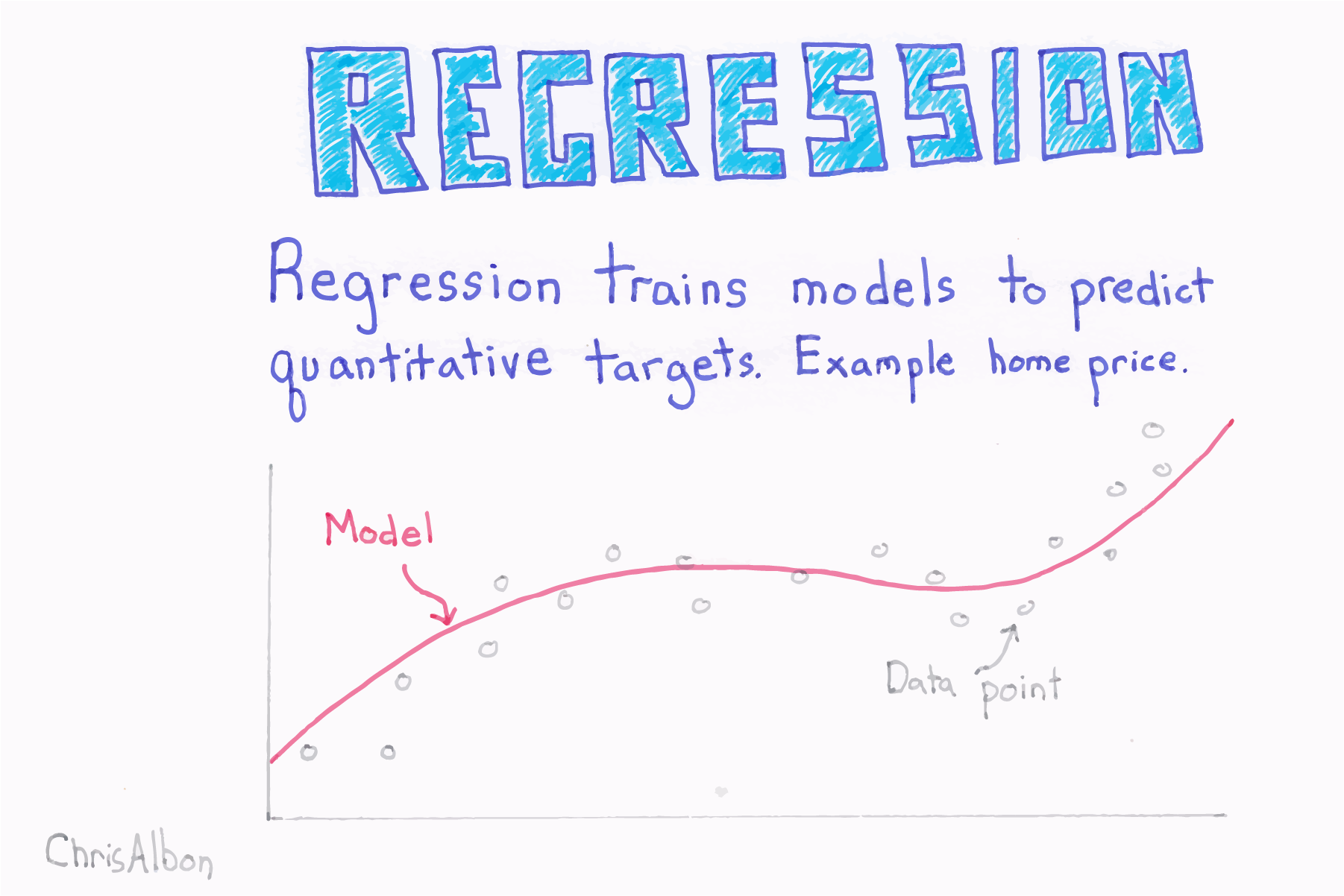
Introduction to Regression

Your goal will be to use this data to predict the life expectancy in a given country based on features such as the country’s GDP, fertility rate, and population.

As always, it is important to explore your data before building models. we have constructed a heatmap showing the correlation between the different features of the Gapminder dataset, which has been pre-loaded into a DataFrame as df

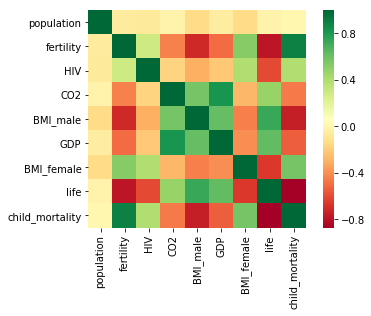
Cells that are in green show positive correlation, while cells that are in red show negative correlation.

### Import packages
import numpy as np
import pandas as pd
import seaborn as sns

# Read the CSV file into a DataFrame : df & check it
df = pd.read_csv("./data/gm_2008_region.csv")
df.head()

df.info()

df.describe()

# computes the pairwise correlation between columns
sns.heatmap(df.corr(), square=True, cmap='RdYlGn')

Since the target variable here is quantitative, this is a regression problem. To begin, you will fit a linear regression with just one feature: 'fertility' , which is the average number of children a woman in a given country gives birth to. In later exercises, you will use all the features to build regression models. Before that, however, you need to import the data and get it into the form needed by scikit-learn. This involves creating feature and target variable arrays. Furthermore, since you are going to use only one feature to begin with, you need to do some reshaping using NumPy’s .reshape() method.

The basic of linear regression

• y = ax + b
  • y = target
  • x = single feature
  • a, b = parameters of model
• How do we choose a and b ?
• Define an error function for any given line
  • choose the line that minimizes the error function
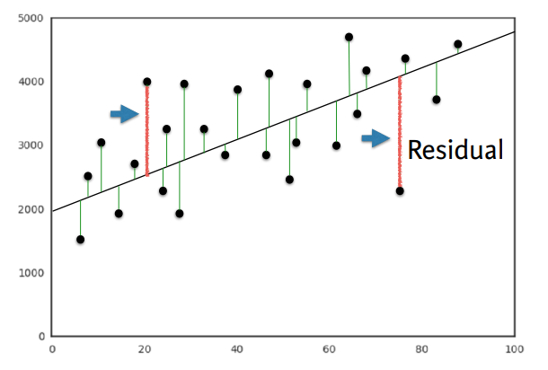
• OLS(Ordinary Least Squares) : Minimize sum of squares of residuals
  
• Linear regression in higher dimensions
  • \[y = a_{1}x_{1} + a_{2}x_{2} + b\]
  • To fit a linear regression model here :
    • need to specify 3 variables
  • In higher dimensions :
    • \[y = a_{1}x_{1} + a_{2}x_{2} + a_{n}x_{n} + b\]
    • Must specify coefficient for each feature and the variable b
  • Scikit-learn API works exactly the same way:
    • Pass two arrays : Features, and target

Fit & predict for regression

Now, you will fit a linear regression and predict life expectancy using just one feature. you will use the fertility feature of the Gapminder dataset. Since the goal is to predict life expectancy, the target variable here is life.

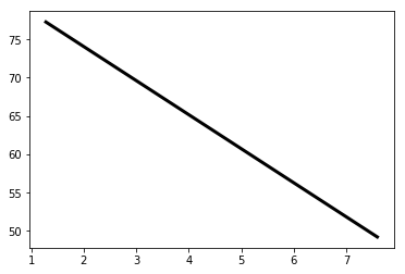
A scatter plot with fertility on the x-axis and life on the y-axis has been generated. As you can see, there is a strongly negative correlation, so a linear regression should be able to capture this trend. Your job is to fit a linear regression and then predict the life expectancy, overlaying these predicted values on the plot to generate a regression line. You will also compute and print the \(R^{2}\) score using sckit-learn’s .score() method.

# Import LinearRegression
from sklearn.linear_model import LinearRegression

X_fertility = df["fertility"].values.reshape(-1,1)
y = df["life"].values.reshape(-1,1)

# Create the regressor: reg
reg = LinearRegression()

# Create the prediction space
prediction_space = np.linspace(min(X_fertility), max(X_fertility)).reshape(-1,1)

# Fit the model to the data
reg.fit(X_fertility, y)

# Compute predictions over the prediction space: y_pred
y_pred = reg.predict(prediction_space)

# Print R^2 
print(reg.score(X_fertility, y))

# Plot regression line
plt.plot(prediction_space, y_pred, color='black', linewidth=3)
plt.show()

Train/test split for regression

Train and test sets are vital to ensure that your supervised learning model is able to generalize well to new data. This was true for classification models, and is equally true for linear regression models.

you will split the Gapminder dataset into training and testing sets, and then fit and predict a linear regression over all features. In addition to computing the \(R^{2}\) score, you will also compute the Root Mean Squared Error (RMSE), which is another commonly used metric to evaluate regression models.

# Import necessary modules
from sklearn.linear_model import LinearRegression
from sklearn.metrics import mean_squared_error
from sklearn.model_selection import train_test_split

y = df.pop("life")
df.drop("Region", axis=1, inplace=True) # Region culumn has text data
X = df.values.reshape(-1,8)
y = y.values.reshape(-1,1)

# Create training and test sets
X_train, X_test, y_train, y_test = train_test_split(X, y, test_size = 0.3, random_state=42)

# Create the regressor: reg_all
reg_all = LinearRegression()

# Fit the regressor to the training data
reg_all.fit(X_train, y_train)

# Predict on the test data: y_pred
y_pred = reg_all.predict(X_test)

# Compute and print R^2 and RMSE
print("R^2: {}".format(reg_all.score(X_test, y_test)))
rmse = np.sqrt(mean_squared_error(y_test, y_pred))
print("Root Mean Squared Error: {}".format(rmse))

Cross Validation

• Model performance is dependent on way the data is split
• Not representative of the model’s ability to generalize
• Solution : Cross Validation

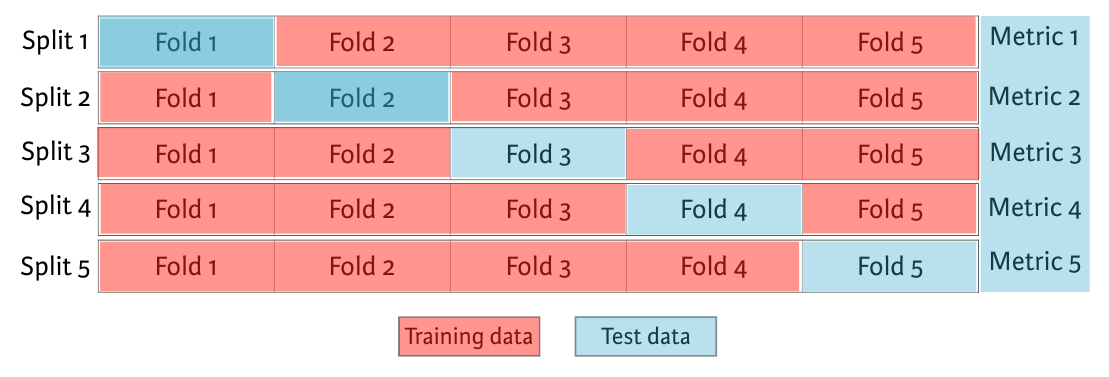
For instances, We begin by splitting the dataset into five groups or folds. Then, we hold out the first fold as a test set, fit our model on the remaining four folds, predict on the test set, and compute the metric of interest. Next, we hold out second fold as our test set, fit on the remaining data, predict on the test set, and compute the metric of interest. Then, similarly with the third, fourth and fifth fold. As a result, we get five values of R squared from which we can compute statics of interest. As we split the dataset into five folds, we call this process 5-fold cross validation. If you use 10 folds, it is called 10-fold cross validation. More generally, if you use k folds, it is called k-fold cross validation or k-fold CV.

• 5 folds = 5-fold CV
• k folds = k-fold CV
• More folds = More computationally expensive
  • fittings and predicting more times.

5-fold cross validation

Cross-validation is a vital step in evaluating a model. It maximizes the amount of data that is used to train the model, as during the course of training, the model is not only trained, but also tested on all of the available data. you will practice 5-fold cross validation on the Gapminder data. By default, scikit-learn’s cross_val_score() function uses \(R_{2}\) as the metric of choice for regression. Since you are performing 5-fold cross-validation, the function will return 5 scores. Your job is to compute these 5 scores and then take their average.

# Import the necessary modules
from sklearn.linear_model import LinearRegression
from sklearn.model_selection import cross_val_score

# Create a linear regression object: reg
reg = LinearRegression()

# Compute 5-fold cross-validation scores: cv_scores
cv_scores = cross_val_score(reg, X, y, cv=5)

# Print the 5-fold cross-validation scores
print(cv_scores)

print("Average 5-Fold CV Score: {}".format(np.mean(cv_scores)))

[0.81720569 0.82917058 0.90214134 0.80633989 0.94495637]
Average 5-Fold CV Score: 0.8599627722793507

K-fold Cross validation

Cross validation is essential but do not forget that the more folds you use, the more computationally expensive cross-validation becomes. Your job is to perform 3-fold cross-validation and then 10-fold cross-validation on the Gapminder dataset. you can use %timeit to see how long each 3-fold CV takes compared to 10-fold CV by executing the following cv=3 and cv=10.

%timeit cross_val_score(reg, X, y, cv = ____)

# Import necessary modules
from sklearn.linear_model import LinearRegression
from sklearn.model_selection import cross_val_score

# Create a linear regression object: reg
reg = LinearRegression()

# Perform 3-fold CV
cvscores_3 = cross_val_score(reg, X, y, cv=3)
print(np.mean(cvscores_3))

# Perform 10-fold CV
cvscores_10 = cross_val_score(reg,X, y, cv=10)
print(np.mean(cvscores_10))