Information Theory (Entropy, KL Divergence, Cross Entropy)

2018, Oct 13    

• 아래 내용은 정보 이론 중 Entropy, Cross Entropy, KL Divergence를 다룬 내용입니다. 기술 블로그 초창기에 적은 글이라서 큰 꿈을 가지고 적었는지 영어로 작성하였네요.

table of contents

• What is information?

• What is the entropy?

• What is the KL divergence?

• Mutual information with KL divergence

• Is order important in KL divergence?

• What is the Cross Entropy?

What is information?

• Let’s think about two cases. Which case does have more information?

• ① It’s clear today. In the news, it will be clear tomorrow too.
• ② It’s clear today. But in the news, it will be heavy rainy tomorrow.

• In the first case, probability of clear in tomorrow is high because today is clear. Intuitively, we get less information.
• On the contrary, probability of second case is low. But we get information a lot. By this simple example, we can figure out that probability and information gain has inverse proportional relation.
• For this reason, information gain can be though as alarming rate. For example, If world war 3 happens, we will be alarmed too much. (we gain a lot of data..)

• Basically, an event which happens in low probability makes us alarmed. And it has a lot of data.
• This relation is the main concept of information theory.
• The main function of information theory is quantifying the information and making possible to calculate it. In order to do it, What we can measure is probability.
• we can formulate above example like this.

• \[P(\text{tomorrow} = \text{heavy rainy} \ \vert \ \text{today} = \text{clear})\]
• \[P(\text{tomorrow} = \text{clear} \ \vert \ \text{today} = \text{clear})\]

• Okay! we can define how to measure information quantity when knowing the probability of an event.

• \[h(x) = -\log_{2}{P(x)} \tag{1}\]

• equation (1) shows the answer. \(x\) is random variable.
• In above example, \(x\) is random variable showing clear or rainy. Let me suppose that \(x\) has a specific value. \(P(x)\) is x’s probability and h(x) is the information quantity or, self-information.

• For example, \(x\) has an event e and its probability is \(P(e) = 1/1024\) (only a time happens during 1024 times),
• information quantity is \(-\log_{2}{(1/1024)} = 10 \text{bit}\).
• Extreme case is \(P(e) = 1\). In this extreme case, we can only get the information that e always happens.
• So, we don’t get any alarming information if we additionally get to know that e happens. If we assign the \(P(e) = 1\) into equation (1), information quantity \(h(x) = 0\).
• we can change base 2 to e(natural constant) then, unit is changed from bit to natural.

What is the entropy?

• Entropy is the average of information quantities that random variable \(x\) can have.

• \[H(x) = -\sum_{x}P(x)log_{2}P(x) \tag{2}\]
• \[H(x) = -\int_{\infty}^{\infty} P(x)log_{2}P(x) dx \tag{3}\]

Equation (2) is the entropy of discrete case and (3) is of continuous case.

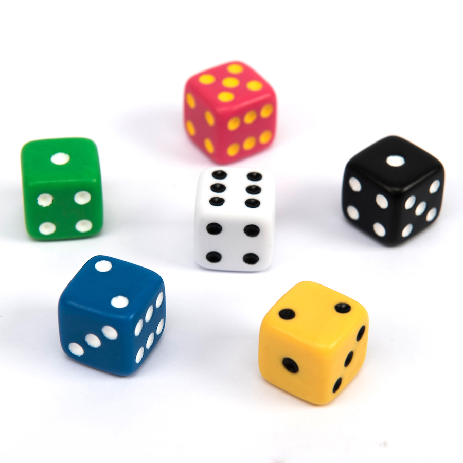
• Let me explain entropy with dice. let random variable x as spot on a die.
• x can have value from 1 to 6(1,2,3,4,5,6) and each has same probability as \(\frac{1}{6}\). Accordingly, entopy is 2.585 bits.

• \[H(x) = -\sum\frac{1}{6}log_{2}\frac{1}{6} = 2.585 bits\]

Thinking about the characteristic of entropy, entropy is maximized when all events which have same probability of occurrence. In other words, the extent of chaos become maximized or uncertainty become maximized. In the dice example, we don’t know which spot will we get and predicting it is very hard. On the other hand, the case of minimum entropy is a event has 1(100%) probability and others have 0(0%) probability. In this case, entropy is 0. uncertainty is nothing. Accordingly, No chaos.

How about this example? This die has special probability of \(P(x=1) = \frac{1}{2}\) and other each event has \(P(x = 2 or 3 or ... 6) = \frac{1}{10}\). Is uncertainty increasing or decreasing comparing to normal die?

Before check it, suppose that there are two cases. each case has two probability distribution with random variable x.

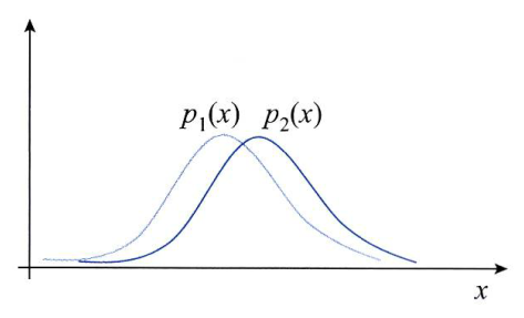
As above example, two probability distributions are largely overlapped. In other words, there are nothing special difference between two.

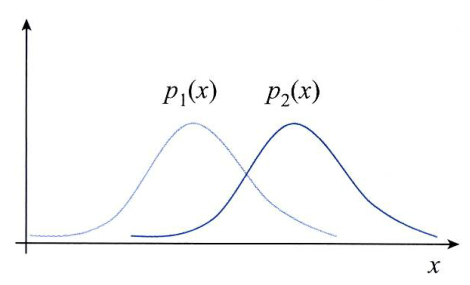
In this case, two probability distributions are little overlapped. Accordingly, They are different.

Then, How can we know the difference as numeric value? In order to quantify the difference, we do it with KL divergence(Kullback-Leibler divergence).

What is the KL divergence?

Let’s look into KL divergence with the above example. we can define KL divergence formula like this.

• \[KL(P_{1}(x), P_{2}(x)) = \sum_{x}P_{1}(x)log_{2}\frac{P_{1}(x)}{P_{2}(x)} \tag{4}\]
• \[KL(P_{1}(x), P_{2}(x)) = \int_{R_{d}}P_{1}(x)log_{2}\frac{P_{1}(x)}{P_{2}(x)}dx \tag{5}\]

Above formulas have range of \(KL(P_{1}(x), P_{2}(x)) \ge 0\) and \(KL(P_{1}(x), P_{2}(x)) = 0\) if \(P_{1}(x) = P_{2}(x)\).
It’s easy right? we can think that it is similar to distance between two distribution. but we just call it divergence because we can not guarantee \(KL(P_{1}(x), P_{2}(x))\) and \(KL(P_{2}(x), P_{1}(x))\) are same. Additionally, we call it as relative entropy.

Okay! then, let’s see another example.

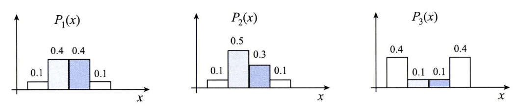
Let random variable x have different probability distribution.

• \(P_{1}(x)\) and \(P_{2}(X)\) have similar distribution and
• \(P_{1}(x)\) and \(P_{3}(X)\) don’t.

Then, calculate KL divergence.

• \[KL(P_{1}(x), P_{2}(x)) = 0.1log_{2}\frac{0.1}{0.1} + 0.4log_{2}\frac{0.4}{0.5} + 0.4log_{2}\frac{0.4}{0.3} + 0.1log_{2}\frac{0.1}{0.1} = 0.037\]
• \[KL(P_{1}(x), P_{3}(x)) = 0.1log_{2}\frac{0.1}{0.4} + 0.4log_{2}\frac{0.4}{0.1} + 0.4log_{2}\frac{0.4}{0.1} + 0.1log_{2}\frac{0.1}{0.4} = 1.200\]

As a result of KL divergence, \(P_{1}(x)\) and \(P_{1}(x)\) is close (0.037) and \(P_{1}(x)\) and \(P_{3}(x)\) are farther (1.200) than former.

Mutual information with KL divergence

With KL divergence, we can see the mutual information between two random variable x and y. Mutual information indicates how much two variables are dependent. Let me suppose that random variable x and y are have distribution of p(x) and p(y). if x and y are independent, p(x, y) = p(x)p(y). Accordingly, they don’t have any dependency. On the other hand, if difference between joint distribution p(x, y) and p(x)p(y) is larger and larger, they become more dependent. Thus, KL divergence of p(x,y) and p(x)p(y) measures dependency of x and y.

• \[I(x,y) = KL(P(x,y) P(x)P(y)) = \sum_{x}\sum_{y}P(x,y)log_{2}\frac{P(x,y)}{P(x)P(y)} \tag{6}\]
• \[I(x,y) = KL(P(x,y), P(x)P(y)) = \int^{\infty}_{\infty}\int^{\infty}_{\infty} P(x,y)log_{2}\frac{P(x,y)}{P(x)P(y)} \tag{7}\]

In the classification problems, Which state is better that KL divergence is large or small? Answer is Large. If KL divergence is large then, their distribution is far apart and it is easy to classify.

If you add new features, then calculate the KL divergence between old feature data and new one. If the value is too small, they are dependent and maybe not useful.

Is order important in KL divergence?

In KL divergence of \(KL(P_{1}(x), P_{2}(x))\), many use \(P_{1}(x)\) as Label or True, \(P_{2}(x)\) as Prediction.

• \[KL(P_{1}(x), P_{2}(x)) = \sum_{x}P_{1}(x)log_{2}\frac{P_{1}(x)}{P_{2}(x)}\]

In a point of \(P_{1}(x) = 0\), regardless of \(P_{2}(x)\), values is zero. That is, don’t care the prediction(estimation) in a point where true value doesn’t exist.

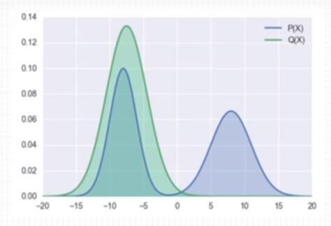
If P(x) = Label, Q(x) = Prediction then, greater than about 3 value points will be zero in KL divergence. Because In terms of \(\sum_{x}P(x)log_{2}\frac{P(x)}{Q(x)}\), P(x) is zero.

On the other hand, In Reverse KL divergence, don’t care the point where prediction value doesn’t exist.

• \[KL(P_{2}(x), P_{1}(x)) = \sum_{x}P_{2}(x)log_{2}\frac{P_{2}(x)}{P_{1}(x)} , where P_{1}(x) = Label, P_{2}(x) = Prediction\]

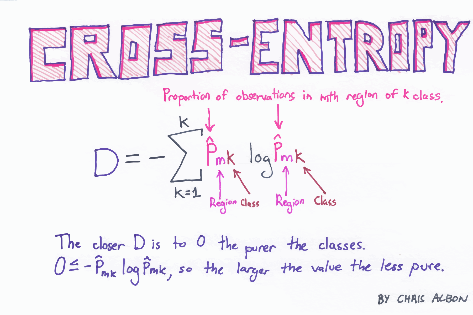
What is the Cross Entropy?

If you study Neural Network then, you maybe know the cross entropy. we usually use it as loss function. As you may know, we used cross entropy in the KL divergence.

• Let’s look into CE (Cross Entropy)

• Entropy :

• \[H(x) = -\sum_{x}P(x)log_{2}P(x) \tag{2}\]

• KL divergence :

• \[KL(P_{1}(x), P_{2}(x)) = \sum_{x}P_{1}(x)log_{2}\frac{P_{1}(x)}{P_{2}(x)} \tag{4}\]

• Cross Entropy :

• \[H(P_{1}(x), P_{2}(x)) = \sum_{x}P_{1}(x)log_{2}\frac{1}{P_{2}(x)} = -\sum_{x}P_{1}(x)log_{2}P_{2}(x)\]

• Yes it is! CE is the negative part of KL divergence.
• KL divergence = Entropy + Cross Entropy
• What is the \(P_{1}(x)\) and \(P_{2}(x)\) in usual?
• \(P_{1}(x)\) is label(True value) and \(P_{2}(x)\) is Prediction.
• Oh, Do you get feel for the reason why we use CE as loss function?
• Actually KL divergence and CE has same meaning in loss function(don’t need entropy). Therefore we use CE.

For example, in the binary classification problem, you have ever used it as loss function. (In above, we used \(log_{2}\) but in neural network, usually use \(ln = log_{e}\))

• \[a = \sigma(z), z = wx + b\]
• \[\mathcal L = -\frac{1}{n}\sum_{x}[ylna + (1-y)ln(1-a)]\]
• \[\frac{\partial\mathcal L}{\partial w_{j}} = -\frac{1}{n}\sum_{x}(\frac{y}{\sigma(z)} - \frac{(1-y)}{1-\sigma(z)})\frac{\partial\sigma}{\partial w_{j}}\]
• \[= \frac{\partial\mathcal L}{\partial w_{j}} = -\frac{1}{n}\sum_{x}(\frac{y}{\sigma(z)} - \frac{(1-y)}{1-\sigma(z)})\sigma^{'}(z)x_{j}\]
• \[= \frac{1}{n}\sum_{x}\frac{\sigma^{'}(z)x_{j}}{\sigma(z)(1-\sigma(z))}(\sigma(z)-y)\]
• \[= \frac{1}{n}\sum_{x}x_{j}(\sigma(z) - y)\]

That’s it! we have look through Entropy, KL divergence and Cross Entropy.

If you have question, feel free to ask me.

Reference

• 패턴 인식(Pattern Recognition) 오일석
• KL-divergence from Terry TaeWoong Um