마할라노비스 거리(Mahalanobis distance)
2020, Feb 01
- 참조 : 패턴인식 (오일석)
- 이번 글에서는 마할라노비스 거리에 대하여 다루어 보도록 하겠습니다.
마할라노비스 거리의 정의
- 이 글을 정확하게 이해하려면 가우시안 분포와 분별 함수에 대한 이해가 필요합니다.
- 위의 링크인 가우시안 분포와 분별 함수를 살펴보겠습니다. 어떤 분포를 가우시안 분포로 가정하였을 때,
likelihood를 표현하면 다음과 같습니다.
- \[p(x \vert w_{i}) = N(\mu_{i}, \Sigma_{i}) = \frac{1}{(2\pi)^{d/2} \vert \Sigma_{i} \vert ^{1/2}} \text{exp} (-\frac{1}{2}(x - \mu_{i})^{T} \Sigma_{i}^{-1}(x - \mu_{i}))\]
- 베이지안 확률에서 관심이 있는
posterior를 구하기 위해 위에서 구한likelihood에prior를 곱하여posterior를 만들어 보겠습니다. - 이 때, 단조 증가 함수의 성질을 이용하여
log를 씌우겠습니다.
- \[g_{i}(x) = \text{ln}(f(x)) = \text{ln}(p(x \vert w_{i})P(w_{i})) = \text{ln}(N(\mu_{i}, \Sigma_{i})) + \text{ln}(P(w_{i}))\]
- \[= -\frac{1}{2}(x - \mu_{i})^{T}\Sigma_{i}^{-1}(x - \mu_{i}) - \frac{d}{2}\text{ln}(2\pi) - \frac{1}{2}\text{ln}(\vert \Sigma_{i} \vert) + \text{ln}(P(w_{i}))\]
- 위 식을 좀 더 간단하게 정리하기 위하여 클래스 별
prior와covariance가 동일하다고 가정하면 위 식에서 \(- \frac{d}{2}\text{ln}(2\pi) - \frac{1}{2}\text{ln}(\vert \Sigma_{i} \vert) + \text{ln}(P(w_{i}))\) 부분은 모두 상수가 되기 때문에 소거가 가능하여 최종 식은 다음과 같습니다.
- \[g_{i}(x) = -\frac{1}{2}(x - \mu_{i})^{T}\Sigma_{i}^{-1}(x - \mu_{i})\]
- 위 식은
posterior이므로 \(g_{i}(x)\)의 값이 가장 큰 클래스를 선택하는 것이 식의 최종 목적이 됩니다. - 그 말은 (위 식에 마이너스가 있으므로) \((x - \mu_{i})^{T}\Sigma_{i}^{-1}(x - \mu_{i})\) 이 가장 작은 클래스가 가장 큰
posterior를 가지게 됩니다. - 이 때, 이 term이 바로 마할라노비스 거리가 됩니다.
- 마할라노비스 거리 : \(\Biggl( (x - \mu_{i})^{T}\Sigma_{i}^{-1}(x - \mu_{i}) \Biggr)^{0.5}\)
- 유클리디안 거리 : \(\Biggl( (x - \mu_{i})^{T}(x - \mu_{i}) \Biggr)^{0.5}\)
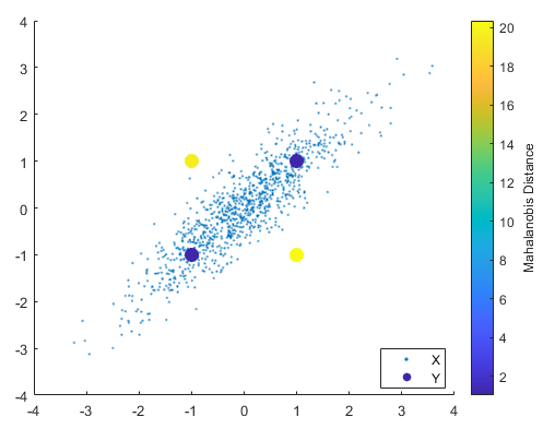
- 즉, 위 식을 보면 마할라노비스 거리는 \(x\) 에서 \(\mu_{i}\) 까지의 거리가 됩니다. 좀 더 정확히 말하면 \(x\)에서 정규 분포 \(N(\mu_{i}, \Sigma)\) 까지의 거리입니다.
- 기존에 알고 있던 유클리디안 거리에 공분산 계산이 더해진 것으로도 이해할 수 있습니다. 만약 \(\Sigma = \sigma^{2} I\)인 형태라면 즉, 각 클래스 간의 공분산이 모두 0인 상태라면 마할라노비스 거리는 유클리디안 거리와 동일합니다.
- 따라서 마할라노비스 거리에서는 공분산이 중요한 역할을 합니다.
마할라노비스 거리 예제
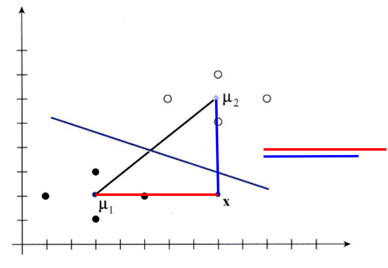
- 위 그림을 보면 점 \(x\)와 \(\mu_{1}, \mu_{2}\)를 중심으로 하는 두 분포가 있습니다.
- 먼저 유클리디안 거리를 이용하여 분포의 평균과 비교하면 점 \(x\)는 \(\mu_{2}\)을 중심으로 하는 분포와 더 가깝습니다. 직선 거리를 보시면 쉽게 알 수 있습니다.
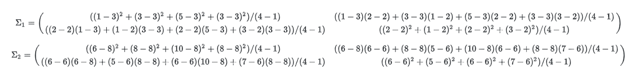
- 공분산은 위 식과 같이 구할 수 있습니다. 관련 식은 가우시안 분포와 분별 함수에서 살펴보시기 바랍니다.
- \[\Sigma = \begin{pmatrix} 8/3 & 0 \\ 0 & 2/3 \end{pmatrix}\]
- 먼저 \(\mu_{1}\) 까지의 마할라노비스 거리를 구해보겠습니다.
- \[\Biggl( \begin{pmatrix} 8 - 3 & 2 - 2 \end{pmatrix} \begin{pmatrix} 3/8 & 0 \\ 0 & 3/2 \end{pmatrix} \begin{pmatrix} 8 - 3 \\ 2 - 2 \end{pmatrix} \Biggr)^{1/2} = 3.062\]
- 다음은 \(\mu_{2}\) 까지의 마할라노비스 거리를 구해보겠습니다.
- \[\Biggl( \begin{pmatrix} 8 - 8 & 2 - 6 \end{pmatrix} \begin{pmatrix} 3/8 & 0 \\ 0 & 3/2 \end{pmatrix} \begin{pmatrix} 8 - 8 \\ 2 - 6 \end{pmatrix} \Biggr)^{1/2} = 4.899\]
- 따라서 유클리디안 거리를 이용하였을 때에는 \(\mu_{2}\)가 더 가까웠지만 마할라노비스 거리를 이용하였을 때에는 \(\mu_{1}\)이 더 가까운 것을 알 수 있습니다.
- 직관적으로 해석하면 두 정규 분포 모두 가로 방향으로 퍼져있고 세로 방향으로는 조밀하게 분포되어 있습니다. 즉, 가로 방향으로의 분산은 크고 세로 방향으로의 분산은 작습니다. 가로 방향으로의 분산이 크기 때문에 분산을 거리의 기준으로 생각하면 실제로 생각하는 것 보다 더 거리는 가깝게 느낄 수 있습니다. 반면 세로 방향으로의 분산은 작기 때문에 실제로 생각하는 것 보다 더 멀게 느껴질 수 있습니다.
- 따라서 점 \(x\)가 \(\mu_{1}\)과는 가로 방향에 위치하므로 마할라노비스 거리 상에서는 더 가깝다고 직관적으로 이해할 수도 있습니다.
마할라노비스 거리 코드 예제
- 마할라노비스 거리를 구할 때에는 공분산 행렬을 미리 구해놓으면 된다는 점에서 유클리디안 거리를 이용하는 것과 차이점이 있었습니다. 즉, 구하고자 하는 데이터들의 공분산을 미리 구해놓고 앞에서 설명한 바와 같이 마할라노비스 거리를 구하면 됩니다. 아래 코드의
all_points는 3D 포인트 (X, Y, Z)를 (N, 3) 행렬에 저장하였을 때 기준입니다.
combined_cov_matrix = np.cov(all_points.T)
combined_cov_inv = np.linalg.inv(combined_cov_matrix)

# Function to calculate Mahalanobis distance
def mahalanobis_distance(x, y, cov_inv):
    delta = x - y
    return np.sqrt(delta.T @ cov_inv @ delta)
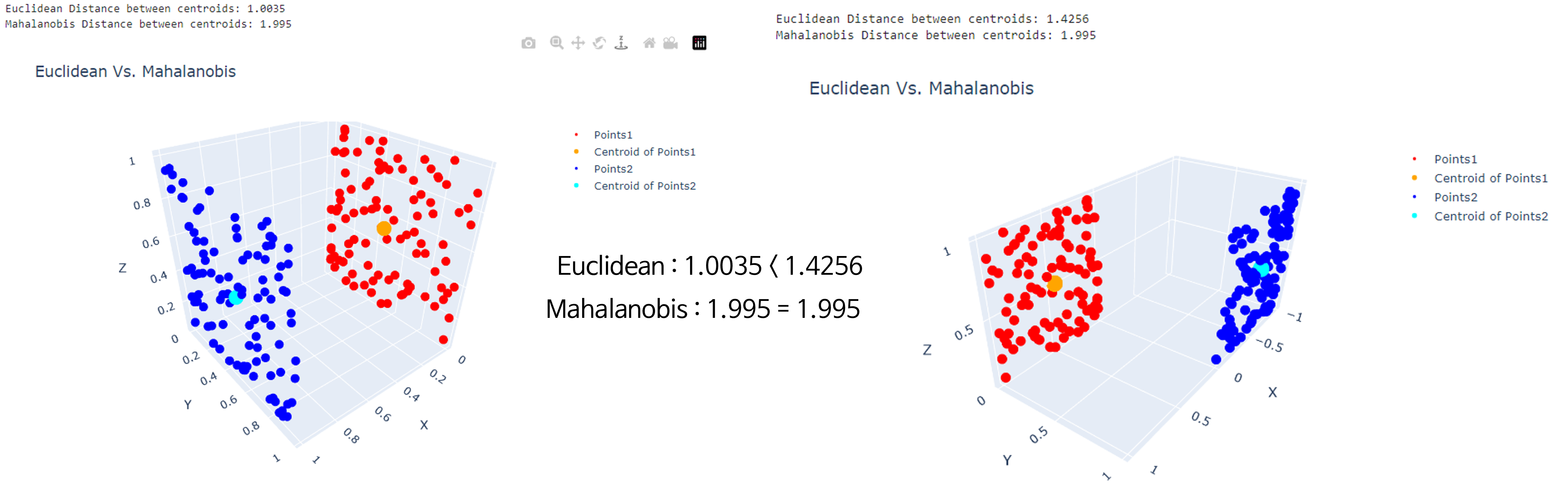
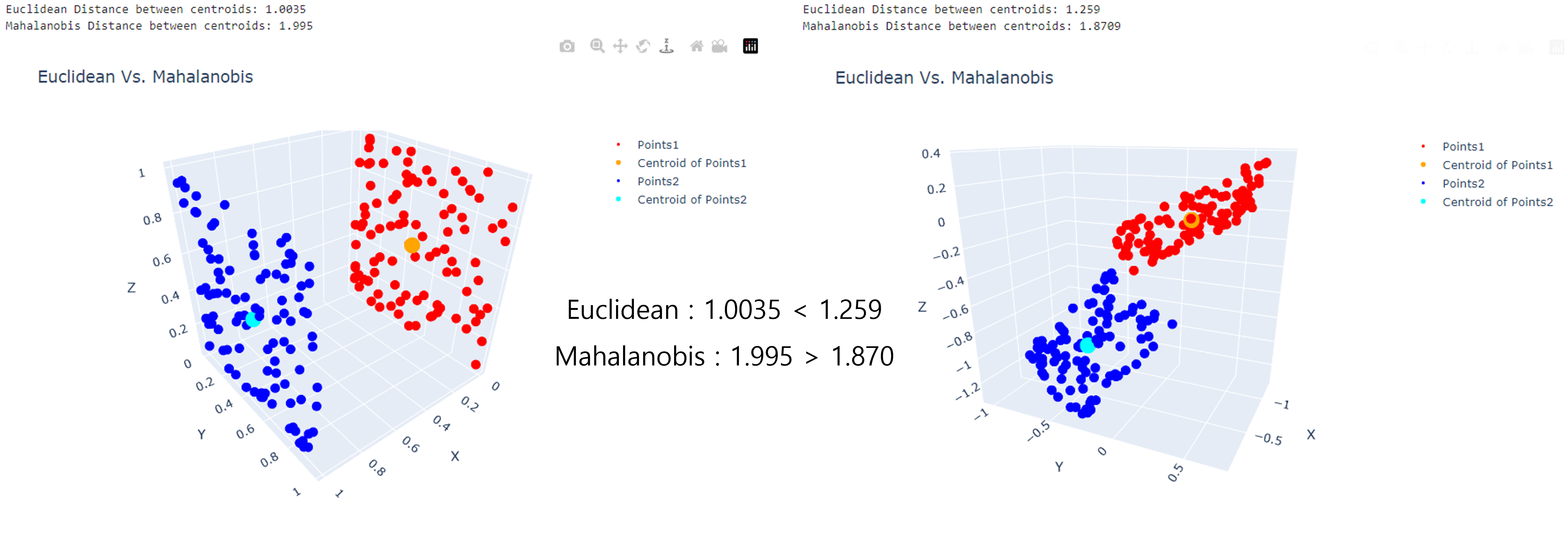
- 지금부터 2가지 경우를 살펴보도록 하겠습니다. 첫번째는
Euclidean Distance는 차이가 있으나Mahalanobis Distance는 차이가 없는 경우 입니다. 이 경우는 데이터가 분포된 방향이 같은 패턴이기 때문에Mahalanobis Distance에는 차이가 없습니다. - 아래 그림에서
Distance는 주황색 점과 청록색 점의 거리를 의미하며 주황색 점은 빨간색 점들의 중앙점이고, 청록색 점은 파란색 점들의 중앙점입니다.
import numpy as np
import matplotlib.pyplot as plt
import plotly.graph_objects as go

# Function to generate points on a plane
def generate_plane_points(mean, normal, n=100, noise_level=0.001):
    # Generate random points
    points = np.random.rand(n, 3)
    # Adjust points to lie on a given plane
    for i in range(n):
        points[i] = points[i] - np.dot(points[i] - mean, normal) * normal
        # Add some noise
        points[i] += np.random.normal(scale=noise_level, size=3)
    return points

# Function to calculate Mahalanobis distance
def mahalanobis_distance(x, y, cov_inv):
    delta = x - y
    return np.sqrt(delta.T @ cov_inv @ delta)

# Define two planes
mean1 = np.array([0, 0, 0])
normal1 = np.array([1, 0, 0])
points1 = generate_plane_points(mean1, normal1)

mean2 = np.array([1, 0, 0])
normal2 = np.array([-1, 0, 0])
points2= generate_plane_points(mean2, normal2)

# Extract x, y, and z coordinates from points1
x1 = points1[:, 0]
y1 = points1[:, 1]
z1 = points1[:, 2]

# Extract x, y, and z coordinates from points2
x2 = points2[:, 0]
y2 = points2[:, 1]
z2 = points2[:, 2]

# Calculate the combined covariance matrix of the two groups
all_points = np.vstack([points1, points2])
combined_cov_matrix = np.cov(all_points.T)
combined_cov_inv = np.linalg.inv(combined_cov_matrix)

# Calculate Mahalanobis distance between centroids
centroid1_mean = np.mean(points1, axis=0)
centroid2_mean = np.mean(points2, axis=0)
distance_between_centroids = mahalanobis_distance(centroid1_mean, centroid2_mean, combined_cov_inv)

# Output the distance
print("Euclidean Distance between centroids:", round(np.linalg.norm(centroid1_mean - centroid2_mean), 4))
print("Mahalanobis Distance between centroids:", round(distance_between_centroids, 4))

# Create a 3D scatter plot for points1 (red)
trace1 = go.Scatter3d(x=x1, y=y1, z=z1, mode='markers', marker=dict(size=3, color='red'), name='Points1')
trace1_mean = go.Scatter3d(x=centroid1_mean[0:1], y=centroid1_mean[1:2], z=centroid1_mean[2:3], mode='markers', marker=dict(size=5, color='orange'), name='Centroid of Points1')
# Create a 3D scatter plot for points2 (blue)
trace2 = go.Scatter3d(x=x2, y=y2, z=z2, mode='markers', marker=dict(size=3, color='blue'), name='Points2')
trace2_mean = go.Scatter3d(x=centroid2_mean[0:1], y=centroid2_mean[1:2], z=centroid2_mean[2:3], mode='markers', marker=dict(size=5, color='cyan'), name='Centroid of Points2')

# Create the figure and add the traces
fig = go.Figure(data=[trace1,trace1_mean, trace2, trace2_mean])

# Customize the layout
fig.update_layout(scene=dict(xaxis_title='X', yaxis_title='Y', zaxis_title='Z'),
                  title='Euclidean Vs. Mahalanobis',
                  width=800, height=600)

# Display the plot
fig.show()

# Apply transformation to second plane (e.g., rotation)
theta1 = np.radians(-90)  # Rotation angle around z axis
rotation_matrix1 = np.array([
    [np.cos(theta1), -np.sin(theta1), 0],
    [np.sin(theta1), np.cos(theta1), 0],
    [0, 0, 1]
])

theta2 = np.radians(90)  # Rotation angle around z axis
rotation_matrix2 = np.array([
    [np.cos(theta2), -np.sin(theta2), 0],
    [np.sin(theta2), np.cos(theta2), 0],
    [0, 0, 1]
])


points1_transformed = rotation_matrix1 @ points1.T # np.dot(points1 - centroid1_mean, rotation_matrix) + centroid1_mean
# points1_transformed = points1.T # np.dot(points1 - centroid1_mean, rotation_matrix) + centroid1_mean
points2_transformed = rotation_matrix2 @ points2.T # np.dot(points2 - centroid2_mean, rotation_matrix) + centroid2_mean

points1_transformed = points1_transformed.T
points2_transformed = points2_transformed.T

x1 = points1_transformed[:, 0]
y1 = points1_transformed[:, 1]
z1 = points1_transformed[:, 2]

x2 = points2_transformed[:, 0]
y2 = points2_transformed[:, 1]
z2 = points2_transformed[:, 2]

# Calculate the combined covariance matrix of the two groups
all_points = np.vstack([points1_transformed, points2_transformed])
combined_cov_matrix = np.cov(all_points.T)
combined_cov_inv = np.linalg.inv(combined_cov_matrix)

# Calculate Mahalanobis distance between centroids
centroid1_mean = np.mean(points1_transformed, axis=0)
centroid2_mean = np.mean(points2_transformed, axis=0)
distance_between_centroids = mahalanobis_distance(centroid1_mean, centroid2_mean, combined_cov_inv)

# Output the distance
print("Euclidean Distance between centroids:", round(np.linalg.norm(centroid1_mean - centroid2_mean), 4))
print("Mahalanobis Distance between centroids:", round(distance_between_centroids, 4))

# Create a 3D scatter plot for points1 (red)
trace1 = go.Scatter3d(x=x1, y=y1, z=z1, mode='markers', marker=dict(size=3, color='red'), name='Points1')
trace1_mean = go.Scatter3d(x=centroid1_mean[0:1], y=centroid1_mean[1:2], z=centroid1_mean[2:3], mode='markers', marker=dict(size=5, color='orange'), name='Centroid of Points1')
# Create a 3D scatter plot for points2 (blue)
trace2 = go.Scatter3d(x=x2, y=y2, z=z2, mode='markers', marker=dict(size=3, color='blue'), name='Points2')
trace2_mean = go.Scatter3d(x=centroid2_mean[0:1], y=centroid2_mean[1:2], z=centroid2_mean[2:3], mode='markers', marker=dict(size=5, color='cyan'), name='Centroid of Points2')

# Create the figure and add the traces
fig = go.Figure(data=[trace1,trace1_mean, trace2, trace2_mean])

# Customize the layout
fig.update_layout(scene=dict(xaxis_title='X', yaxis_title='Y', zaxis_title='Z'),
                  title='Euclidean Vs. Mahalanobis',
                  width=800, height=600)

# Display the plot
fig.show()
- 두번째는
Euclidian Distance와Mahalanobis Distance의 대소 관계가 역전되는 경우 입니다. 아래 오른쪽 그림에서 빨간색과 파란색 점들의 위 아래 분포 방향에 대한 밀도가 상대적으로 높아Mahalanobis Distance가 더 작게 형성된 것을 알 수 있습니다.
# Apply transformation to second plane (e.g., rotation)
# theta1 = np.radians(45)  # Rotation angle around z axis
rotation_matrix1 = np.array(
    [[ 0.24509598, -0.83793063, -0.48764763],
     [ 0.58008904, -0.27626779,  0.76627202],
     [-0.77680413, -0.47068924,  0.41836226]]
)

rotation_matrix2 = np.array(
    [[-0.63465759,  0.57820618, -0.51272542],
     [ 0.22204075, -0.49905858, -0.83763861],
     [-0.74020784, -0.64545963,  0.18834598]
])

points1_transformed = rotation_matrix1 @ points1.T # np.dot(points1 - centroid1_mean, rotation_matrix) + centroid1_mean
# points1_transformed = points1.T # np.dot(points1 - centroid1_mean, rotation_matrix) + centroid1_mean
points2_transformed = rotation_matrix2 @ points2.T # np.dot(points2 - centroid2_mean, rotation_matrix) + centroid2_mean

points1_transformed = points1_transformed.T
points2_transformed = points2_transformed.T

x1 = points1_transformed[:, 0]
y1 = points1_transformed[:, 1]
z1 = points1_transformed[:, 2]

x2 = points2_transformed[:, 0]
y2 = points2_transformed[:, 1]
z2 = points2_transformed[:, 2]

# Calculate the combined covariance matrix of the two groups
all_points = np.vstack([points1_transformed, points2_transformed])
combined_cov_matrix = np.cov(all_points.T)
combined_cov_inv = np.linalg.inv(combined_cov_matrix)

# Calculate Mahalanobis distance between centroids
centroid1_mean = np.mean(points1_transformed, axis=0)
centroid2_mean = np.mean(points2_transformed, axis=0)
distance_between_centroids = mahalanobis_distance(centroid1_mean, centroid2_mean, combined_cov_inv)

# Output the distance
print("Euclidean Distance between centroids:", round(np.linalg.norm(centroid1_mean - centroid2_mean), 4))
print("Mahalanobis Distance between centroids:", round(distance_between_centroids, 4))

# Create a 3D scatter plot for points1 (red)
trace1 = go.Scatter3d(x=x1, y=y1, z=z1, mode='markers', marker=dict(size=3, color='red'), name='Points1')
trace1_mean = go.Scatter3d(x=centroid1_mean[0:1], y=centroid1_mean[1:2], z=centroid1_mean[2:3], mode='markers', marker=dict(size=5, color='orange'), name='Centroid of Points1')
# Create a 3D scatter plot for points2 (blue)
trace2 = go.Scatter3d(x=x2, y=y2, z=z2, mode='markers', marker=dict(size=3, color='blue'), name='Points2')
trace2_mean = go.Scatter3d(x=centroid2_mean[0:1], y=centroid2_mean[1:2], z=centroid2_mean[2:3], mode='markers', marker=dict(size=5, color='cyan'), name='Centroid of Points2')

# Create the figure and add the traces
fig = go.Figure(data=[trace1,trace1_mean, trace2, trace2_mean])

# Customize the layout
fig.update_layout(scene=dict(xaxis_title='X', yaxis_title='Y', zaxis_title='Z'),
                  title='Euclidean Vs. Mahalanobis',
                  width=800, height=600)

# Display the plot
fig.show()