ASPP(Atrous Spatial Pyramid Pooling)

segmentation 글 목록

참조 : https://towardsdatascience.com/review-deeplabv1-deeplabv2-atrous-convolution-semantic-segmentation-b51c5fbde92d
참조 : https://m.blog.naver.com/laonple/221000648527
참조 : https://arxiv.org/abs/1706.05587
참조 : https://towardsdatascience.com/review-deeplabv3-atrous-convolution-semantic-segmentation-6d818bfd1d74
이번 글에서는 segmentation에서 자주 사용되는 ASPP(Atrous Spatial Pyramid Pooling)에 대하여 다루어 보도록 하겠습니다.
ASPP는 DeepLab_v2에서 소개되었고 그 이후에 많은 Segmentation 모델에서 차용해서 사용하고 있습니다.

Atrous convolution

Atrous convolution 또는 dilated convolution에 대한 내용은 제 블로그의 다음 링크를 참조해 주시기 바랍니다. 상당히 자세하게 다루어 놓았습니다.
링크 : https://gaussian37.github.io/dl-concept-dilated_residual_network/

Atrous convolution에 대한 자세한 내용은 위 링크를 참조하시고 이 글을 전개하기 위해 간단하게 살펴보도록 하겠습니다.
1-dimension의 Atrous convolution을 수식으로 나타내면 다음과 같습니다.

\[y[i] = \sum_{k=1}^{K} x[i + r \cdot k]w[k]\]
\[r > 1 \text{ : atrous convolution}, \quad r = 1 \text{ : standard convolution}\]

위 수식에서 \(x\)가 input이고 \(w\)가 filter입니다. 즉, input과 filter를 곱할 때, \(r\)의 값에 따라 얼마나 input을 띄엄 띄엄 선택하여 filter와 곱할 지 결정됩니다.

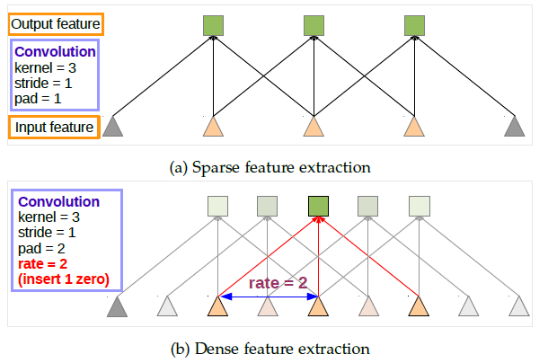
이를 convolution filter에 적용하면 위 그림과 같습니다. 위쪽 그림 (a)가 standard convolution이고 아래쪽 그림 (b)가 atrous convolution을 적용한 형태입니다.
먼저 그림 (a)는 일반적인 convolution 연산입니다. 그리고 기본적으로 사용하는 stride = 1, pad = 1을 사용하여 feature의 크기를 유지하였습니다.
반면 그림 (b)는 이 글에서 설명하는 atrous convolution을 적용한 형태로 필터 간의 거리가 2 인것을 알 수 있습니다. 이 거리의 크기는 r 이라는 상수를 통해 조절됩니다. atrous convolution을 적용할 때, 그림 (a)와 같이 feature의 크기를 유지하려면 stride = 1, pad = r 로 사용하면 됩니다.
같은 크기의 kernel을 사용하였음에도 불구하고 atrous convolution을 적용하였을 때, 더 넓은 범위의 input feature를 cover 할 수 있습니다. 즉, atrous convolution은 input feature의 FOV(Field Of View)를 더 넓게 확장 할 수 있는 장점을 가집니다. 뿐만 아니라 작은 범위의 FOV도 가지기 때문에 다양한 FOV를 다룰 수 있다는 장점을 가집니다.
즉, small FOV를 통한 localization 정확성과 large FOV를 통한 context 이해를 동시에 다룰 수 있게 됩니다.

ASPP(Atrous Spatial Pyramid Pooling) (DeepLab v2)

지금부터 DeepLab v2에서 소개된 ASPP(Atrous Spatial Pyramid Pooling)부터 시작하여 DeepLab v3에서 소개된 ASPP 까지 다루어 보려고 합니다.
먼저 DeepLab v2에서 소개된 ASPP의 구조를 알아보도록 하겠습니다. (pytorch 코드는 성능이 개선된 DeepLab v3의 ASPP를 통해 알아보겠습니다.)

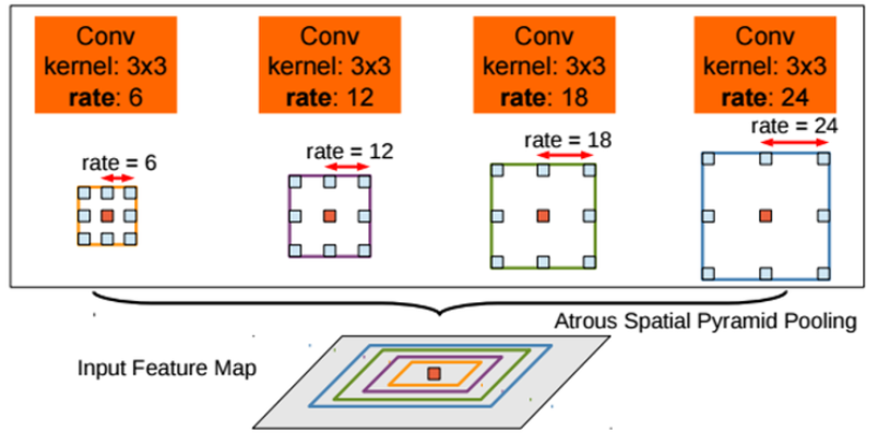
ASPP가 소개된 Deeplab v2에서는 multi-scale에 더 잘 대응할 수 있도록 atrous convolution에 대한 확장 계수를 (6, 12, 18, 24)를 적용하여 위 그림과 같이 합쳐서 사용하였습니다.
Spatial Pyramid Pooling 구조는 SPPNet을 통하여 얻을 수 있었고 이 구조에 atrous convolution을 적용하여 ASPP를 만들었습니다.
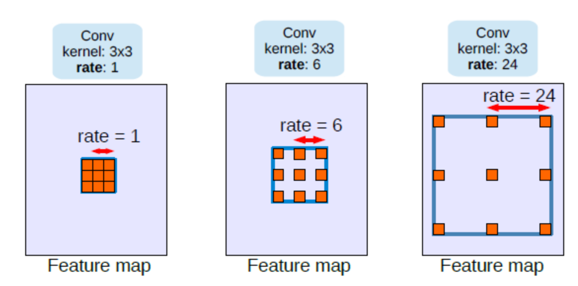
처음 제시되었던 ASPP는 확장 계수 rate를 6 ~ 24 까지 다양하게 변화하면서 다양한 receptive field를 볼 수 있도록 적용하였습니다. 이는 그림 (b)에서 확인할 수 있습니다.
물론 rate가 점점 더 커질 수록 receptive field가 커지는 장점은 있지만 유효한 weight 수가 줄어드는 단점이 있습니다. 여기서 유효한 weight 수 란, zero padding이 된 영역이 아닌 유효한 feature 영역과 연산된 weight를 뜻합니다.

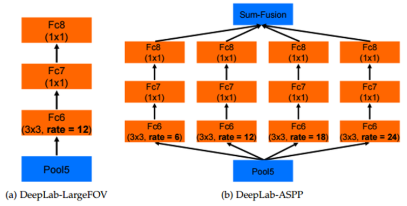
왼쪽 그림은 Deeplab v1의 모델의 일부 layer 형태이고 오른쪽 그림은 Deeplab v2의 layer 형태(ASPP) 입니다.
양쪽 모두 FC6 layer 이전 까지는 동일한 아키텍쳐를 이용하고 있습니다. 하지만 FC6에서 부터 두 모델이 달라집니다.
오른쪽 그림의 Deeplab v2의 경우 ASPP 구조에 확장 계수 6, 12, 18, 24가 적용되어 다양한 스케일을 볼 수 있도록 설계되어 있습니다.
반면 왼쪽 그림의 Deeplab v1의 경우 ASPP 구조와 비교해서 보면 단순히 확장 계수가 12로 고정되어 있다고 생각하면 됩니다.

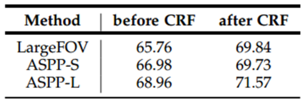
위 성능 지표를 통해 고정된 확장 계수의 ASPP인 Large FOV와 ASPP-S (확장 계수 값이 작은 값들로 구성됨 r = 2, 4, 8, 12) 그리고 ASPP-L (r = 6, 12, 18, 24)를 이용하였을 때의 성능을 비교할 수 있습니다.
그 결과 넓은 multi scale의 receptive field > 좁은 multi scale의 receptive field > 고정된 scale의 receptive field인 것을 확인할 수 있습니다.
따라서 ASPP를 적용할 때 확장 계수는 넓은 multi scale의 receptive field를 사용할 수 있도록 하는 것이 성능을 높일 수 있습니다.

여기 까지 내용을 잘 이해하셨다면 DeepLab v3에서 사용한 ASPP로 넘어가 보도록 하겠습니다. pytorch를 통한 코드 구현은 조금 뒤에 다루어 보려고 합니다. 지금 까지 이해한 내용에서 아주 조금 개념이 추가되면서 성능 개선을 하였기에 성능 열세인 초기의 ASPP 보다는 DeepLab v3 버전의 pytorch 코드를 보는 것이 더 낫다고 판단됩니다.

ASPP(Atrous Spatial Pyramid Pooling) (DeepLab v3)

그럼 지금부터 DeepLab v3에서 개선한 ASPP 내용에 대하여 다루어 보도록 하겠습니다.
먼저 아래 그림을 통해 Multi-Grid Atrous Convolution을 이용하여 더 깊게 layer를 쌓을 수 있는 방법에 대하여 다루어 보도록 하겠습니다.

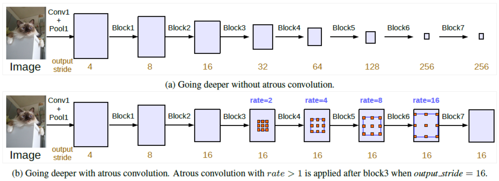
위 그림은 DeepLab_v3에서 소개한 그림입니다. 이 그림을 이해하려면 DeepLab_v3에서 사용한 output_stride 라는 용어를 이해해야 합니다.
output_stride란 입력 이미지의 spatial resolution 대비 최종 출력의 resolution 비율을 뜻합니다. 간단히 말하면 입력 이미지의 height, width의 크기가 어떤 layer의 feature의 heigt, width에 비해 몇 배 큰 지를 나타냅니다.
예를 들어 cityscape 데이터는 (height, width) = (1024, 2048) 입니다. 만약 어떤 layer의 feature가 (64, 128) 이라면 (1024/64, 2048/128) = (16, 16)으로 output_stride = 16이 됩니다.
(a) 와 같은 standard convolution에서는 convolution과 pooling 연산을 거치면서 output_stride가 점점 커지게 됩니다. 반대로 말하면 output feature map의 크기가 점점 더 작아집니다. 이러한 standard convolution 방법은 semantic segmentation에서 다소 불리할 수 있습니다. 왜냐하면 깊은 layer에서는 위치와 공간 정보를 잃을 수 있기 때문입니다. 이 경우 output_stride 수치가 큽니다. 즉, 이 수치가 커진다는 것은 input 대비 feature가 너무 작아졌다는 것을 뜻합니다. 따라서 픽셀 단위의 세세한 정보를 원하는 segmentation에서는 불리하다는 것을 뜻합니다.
반면 (b)와 같이 Atrous Convolution을 적용한 형태에서는 output_stride를 유지할 수 있습니다. 이와 동시에 파라미터의 수나 계산량을 늘리지 않고 더 큰 FOV를 가질 수 있습니다. 그 결과 (a)에 비해 더 큰 output feature map을 만들어 낼 수 있습니다. 따라서 segmentation에 좀 더 유리합니다.

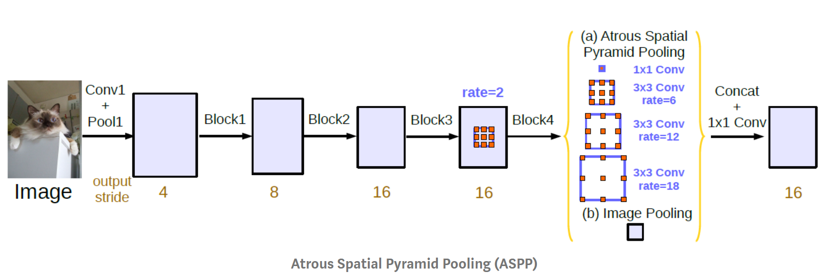
ASPP는 DeepLab_v2에서 소개되었고 그 버전은 앞에서 설명한 형태와 같습니다. v3에서 추가되 내용을 정리해 보면 다음과 같습니다.
batch normalization이 각 convolution 연산에 추가되었습니다. 그리고 deeplab_v3의 구조에서는 output filter의 갯수가 256입니다.
1개의 1x1 convolution과 3개의 3x3 convolution이 각각 6, 12, 18의 rate가 적용되어 사용되었습니다. output_stride가 16인 경우에는 6, 12, 18의 rate가 적용된 반면 output_stride가 8인 경우에는 2배인 12, 24, 36의 rate가 적용되었습니다. deeplab_v2와 비교한다면, deeplabv2에서는 단순히 large FOV를 위해 rate 6, 12, 18, 24를 적용한 구조에 비해 deeplab_v3에서는 1x1 convolution의 추가와 output_stride에 따른 rate의 변화라는 차이점이 있습니다.
각각의 convolution 연산을 거친 branch 들을 모두 concaternation을 하여 합친 다음, 마지막으로 1x1 convolution과 batch normalization을 거쳐서 마무리합니다.
각 branch들의 연산 방법과 branch들을 어떻게 concatenation을 하는 지 정리하면 다음과 같습니다.
① = 1x1 convolution → BatchNorm → ReLu
② = 3x3 convolution w/ rate=6 (or 12) → BatchNorm → ReLu
③ = 3x3 convolution w/ rate=12 (or 24) → BatchNorm → ReLu
④ = 3x3 convolution w/ rate=18 (or 36) → BatchNorm → ReLu
⑤ = AdaptiveAvgPool2d → 1x1 convolution → BatchNorm → ReLu
⑥ = concatenate(① + ② + ③ + ④ + ⑤)
⑦ = 1x1 convolution → BatchNorm → ReLu

ASPP (DeepLab v3) 시각화

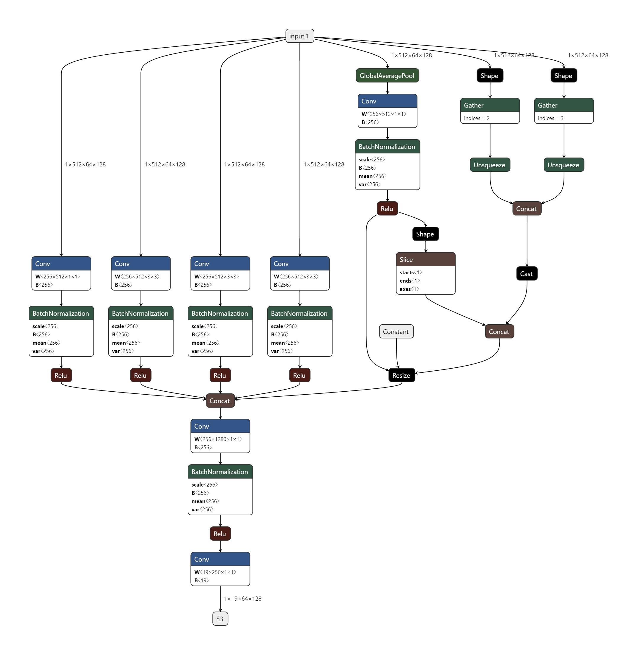
ASPP의 네트워크를 그래프를 통해 시각화 하면 위 그림과 같습니다.
먼저 input의 크기는 (3, 1024, 2048) 크기의 cityscape 데이터를 이용한다고 가정하겠습니다. deeplab_v3의 output_stride가 16인 상태를 가정하면 input 이미지의 크기에 비해 16배 축소된 형태의 feature가 입력으로 들어옵니다. 그리고 feature의 채널 수는 deeplab_v3에서 사용한 그대로 512라고 하겠습니다. 즉, (512, 1024/16, 2048/16) = (512, 64, 128)의 크기의 feature가 입력으로 들어옵니다.
출력은 class의 갯수가 19개라고 가정하였습니다. 따라서 마지막의 출력되는 feature으 크기는 (19, 64, 128)이 됩니다.
위 그림을 자세히 보려면 다음 링크를 클릭하시기 바랍니다.

depplab_v3 구조에 따라서 각 branch의 input channel 수는 512, output channel 수는 256, 최종 class 숫자는 19라고 가정하고 summary를 해보면 다음과 같습니다.

# cityscape 이미지 크기
image_height = 1024
image_width = 2048

# deeplab_v3의 output stride
output_stride = 16

# deeplab_v3의 ASPP 모듈에서 사용된 input 채널 수, output 채널 수
in_channels = 512
out_channels = 256

# 최종 class 수
num_classes = 19

aspp_module = ASPP(in_channels, out_channels, num_classes)
summary(aspp_module, (512, (image_height // output_stride), (image_width // output_stride)))
# ----------------------------------------------------------------
#         Layer (type)               Output Shape         Param #
# ================================================================
#             Conv2d-1         [-1, 256, 64, 128]         131,328
#        BatchNorm2d-2         [-1, 256, 64, 128]             512
#             Conv2d-3         [-1, 256, 64, 128]       1,179,904
#        BatchNorm2d-4         [-1, 256, 64, 128]             512
#             Conv2d-5         [-1, 256, 64, 128]       1,179,904
#        BatchNorm2d-6         [-1, 256, 64, 128]             512
#             Conv2d-7         [-1, 256, 64, 128]       1,179,904
#        BatchNorm2d-8         [-1, 256, 64, 128]             512
#  AdaptiveAvgPool2d-9            [-1, 512, 1, 1]               0
#            Conv2d-10            [-1, 256, 1, 1]         131,328
#       BatchNorm2d-11            [-1, 256, 1, 1]             512
#            Conv2d-12         [-1, 256, 64, 128]         327,936
#       BatchNorm2d-13         [-1, 256, 64, 128]             512
#            Conv2d-14          [-1, 19, 64, 128]           4,883
# ================================================================
# Total params: 4,138,259
# Trainable params: 4,138,259
# Non-trainable params: 0
# ----------------------------------------------------------------
# Input size (MB): 16.00
# Forward/backward pass size (MB): 161.20
# Params size (MB): 15.79
# Estimated Total Size (MB): 192.98
# ----------------------------------------------------------------

결과를 보면 ASPP 모듈의 입력은 (512, 64, 128) 크기의 feature 이고 출력은 (num_class, 64, 128)의 크기로 feature의 입력과 크기는 유지된 것을 확인할 수 있습니다. 즉, output_stride의 크기가 유지되었습니다. deeplab_v2에서는 계속 증가한 output_stride 하였던 단점을 개선하였습니다.
마지막 output feature를 interpolation 하여 원래 intput 이미지 크기로 맞추면 segmentation이 완료됩니다.

Pytorch 코드

import torch
import torch.nn as nn
import torch.nn.functional as F

# ASPP(Atrous Spatial Pyramid Pooling) Module
class ASPP(nn.Module):
    def __init__(self, in_channels, out_channels, num_classes):
        super(ASPP, self).__init__()
        
        # 1번 branch = 1x1 convolution → BatchNorm → ReLu
        self.conv_1x1_1 = nn.Conv2d(in_channels, out_channels, kernel_size=1)
        self.bn_conv_1x1_1 = nn.BatchNorm2d(out_channels)

        # 2번 branch = 3x3 convolution w/ rate=6 (or 12) → BatchNorm → ReLu
        self.conv_3x3_1 = nn.Conv2d(in_channels, out_channels, kernel_size=3, stride=1, padding=6, dilation=6)
        self.bn_conv_3x3_1 = nn.BatchNorm2d(out_channels)

        # 3번 branch = 3x3 convolution w/ rate=12 (or 24) → BatchNorm → ReLu
        self.conv_3x3_2 = nn.Conv2d(in_channels, out_channels, kernel_size=3, stride=1, padding=12, dilation=12)
        self.bn_conv_3x3_2 = nn.BatchNorm2d(out_channels)
    
        # 4번 branch = 3x3 convolution w/ rate=18 (or 36) → BatchNorm → ReLu
        self.conv_3x3_3 = nn.Conv2d(in_channels, out_channels, kernel_size=3, stride=1, padding=18, dilation=18)
        self.bn_conv_3x3_3 = nn.BatchNorm2d(out_channels)

        # 5번 branch = AdaptiveAvgPool2d → 1x1 convolution → BatchNorm → ReLu
        self.avg_pool = nn.AdaptiveAvgPool2d(1)
        self.conv_1x1_2 = nn.Conv2d(in_channels, out_channels, kernel_size=1)
        self.bn_conv_1x1_2 = nn.BatchNorm2d(out_channels)
        
        self.conv_1x1_3 = nn.Conv2d(out_channels * 5, out_channels, kernel_size=1) # (1280 = 5*256)
        self.bn_conv_1x1_3 = nn.BatchNorm2d(out_channels)

        self.conv_1x1_4 = nn.Conv2d(out_channels, num_classes, kernel_size=1)

    def forward(self, feature_map):
        # feature map의 shape은 (batch_size, in_channels, height/output_stride, width/output_stride)

        feature_map_h = feature_map.size()[2] # (== h/16)
        feature_map_w = feature_map.size()[3] # (== w/16)

        # 1번 branch = 1x1 convolution → BatchNorm → ReLu
        # shape: (batch_size, out_channels, height/output_stride, width/output_stride)
        out_1x1 = F.relu(self.bn_conv_1x1_1(self.conv_1x1_1(feature_map)))
        # 2번 branch = 3x3 convolution w/ rate=6 (or 12) → BatchNorm → ReLu
        # shape: (batch_size, out_channels, height/output_stride, width/output_stride)
        out_3x3_1 = F.relu(self.bn_conv_3x3_1(self.conv_3x3_1(feature_map)))
        # 3번 branch = 3x3 convolution w/ rate=12 (or 24) → BatchNorm → ReLu
        # shape: (batch_size, out_channels, height/output_stride, width/output_stride)
        out_3x3_2 = F.relu(self.bn_conv_3x3_2(self.conv_3x3_2(feature_map)))
        # 4번 branch = 3x3 convolution w/ rate=18 (or 36) → BatchNorm → ReLu
        # shape: (batch_size, out_channels, height/output_stride, width/output_stride)
        out_3x3_3 = F.relu(self.bn_conv_3x3_3(self.conv_3x3_3(feature_map)))

        # 5번 branch = AdaptiveAvgPool2d → 1x1 convolution → BatchNorm → ReLu
        # shape: (batch_size, in_channels, 1, 1)
        out_img = self.avg_pool(feature_map) 
        # shape: (batch_size, out_channels, 1, 1)
        out_img = F.relu(self.bn_conv_1x1_2(self.conv_1x1_2(out_img)))
        # shape: (batch_size, out_channels, height/output_stride, width/output_stride)
        out_img = F.upsample(out_img, size=(feature_map_h, feature_map_w), mode="bilinear")

        # shape: (batch_size, out_channels * 5, height/output_stride, width/output_stride)
        out = torch.cat([out_1x1, out_3x3_1, out_3x3_2, out_3x3_3, out_img], 1) 
        # shape: (batch_size, out_channels, height/output_stride, width/output_stride)
        out = F.relu(self.bn_conv_1x1_3(self.conv_1x1_3(out))) 
        # shape: (batch_size, num_classes, height/output_stride, width/output_stride)
        out = self.conv_1x1_4(out) 

        return out

segmentation 글 목록

목차

Atrous convolution

ASPP(Atrous Spatial Pyramid Pooling) (DeepLab v2)

ASPP(Atrous Spatial Pyramid Pooling) (DeepLab v3)

ASPP (DeepLab v3) 시각화

Pytorch 코드

Atrous convolution

ASPP(Atrous Spatial Pyramid Pooling) (DeepLab v2)

ASPP(Atrous Spatial Pyramid Pooling) (DeepLab v3)

ASPP (DeepLab v3) 시각화

Pytorch 코드