Focal Loss (Focal Loss for Dense Object Detection) 알아보기

deep learning 관련 글 목차

• 논문 : https://arxiv.org/pdf/1708.02002.pdf
• 참조 : https://youtu.be/d5cHhLyWoeg
• 참조 : https://www.analyticsvidhya.com/blog/2020/08/a-beginners-guide-to-focal-loss-in-object-detection/
• 참조 : https://towardsdatascience.com/review-retinanet-focal-loss-object-detection-38fba6afabe4

목차

• Focal Loss의 필요성

• Cross Entropy Loss의 문제점

• Balanced Cross Entropy Loss의 한계

• Focal Loss 알아보기

• Focal Loss Pytorch Code

• 이번 글에서는 Focal Loss for Dense Object Detection 라는 논문의 내용을 알아보겠습니다. 이 논문에서는 핵심 내용은 Focal Loss와 이 Loss를 사용한 RetinaNet이라는 Object Detection 네트워크를 소개합니다. 다만, RetinaNet에 대한 내용은 생략하고 Loss 내용에만 집중하도록 하겠습니다.

Focal Loss의 필요성

• Object Detection에는 크게 2가지 종류의 알고리즘이 있습니다. R-CNN 계열의 two-stage detector와 YOLO, SSD 계열의 one-stage detector 입니다.
• one-stage, two-stage detector의 상세 내용은 다음 링크를 참조해 주시기 바랍니다. (https://gaussian37.github.io/vision-detection-table/)
• 간략하게 설명하면 Object Detection은 여러 object들을 Bounding Box를 통해 Localization 즉, 위치를 찾고 Classification 즉, 어떤 물체인지 분류를 하는 작업을 합니다.
• two-stage detector는 먼저 localization을 한 다음에 classification이 순차적으로 이루어지고 one-stage detector는 localization과 classification을 동시에 처리합니다. 정확도 성능으로는 two-stage detector가 좋지만 연산 속도가 오래 걸리는 단점이 있습니다.

• Focal Loss는 one-stage detector의 정확도 성능을 개선하기 위하여 고안되었습니다. one-stage detector가 two-stage detector에 비하여 가지고 있는 문제점은 학습 중 클래스 불균형 문제가 심하다는 것입니다.
• 예를 들어 학습 중 배경에 대하여 박스를 친 것과 실제 객체에 대하여 박스를 친 것의 비율을 살펴보면 압도적으로 배경에 대하여 박스를 친 것이 많다는 것입니다. 학습 중에서 배경에 대한 박스를 출력하면 오류라고 학습이 되지만 그 빈도수가 너무 많다는 것이 학습에 방해가 된다는 뜻입니다. (SSD에서는 학습 시 한 이미지 당 만개 이상의 background에 대한 박스가 있다고 합니다.)
• 이와 같은 문제점이 발생하는 이유는 dense sampling of anchor boxes (possible object locations)로 알려져 있습니다. 예를 들어 RetinaNet에서는 각각의 pyramid layer에서 anchor box가 수천개가 추출됩니다.

• 정리하면 이와 같은 클래스 불균형 문제는 다음 2가지 문제의 원인이 됩니다.
• ① 대부분의 Location은 학습에 기여하지 않는 easy negative이므로 (detector에 의해 background로 쉽게 분류될 수 있음을 의미함) 학습에 비효율적입니다.
• ② easy negative 각각은 높은 확률로 객체가 아님을 잘 구분할 수 있습니다. 즉, 각각의 loss 값은 작습니다. 하지만 비율이 굉장히 크므로 전체 loss 및 gradient를 계산할 때, easy negative의 영향이 압도적으로 커지는 문제가 발생합니다.

• 이러한 문제를 개선하기 위하여 Focal Loss 개념이 도입됩니다.
• Focal Loss는 간단히 말하면 Cross Entropy의 클래스 불균형 문제를 다루기 위한 개선된 버전이라고 말할 수 있으며 어렵거나 쉽게 오분류되는 케이스에 대하여 더 큰 가중치를 주는 방법을 사용합니다. (객체 일부분만 있거나, 실제 분류해야 되는 객체들이 이에 해당합니다.) 반대로 쉬운 케이스의 경우 낮은 가중치를 반영합니다. (background object가 이에 해당합니다.)

Cross Entropy Loss의 문제점

• Cross Entropy Loss의 경우 잘 분류한 경우 보다 잘못 예측한 경우에 대하여 페널티를 부여하는 것에 초점을 둡니다.
• 예를 들어 이진 분류에 대한 Cross Entropy Loss는 다음과 같은 식을 따릅니다.

• \[\text{Cross Entropy Loss} = -Y_{\text{act}} \log{(Y_{pred})} - (1 - Y_{\text{act}})\log{(1 - Y_{\text{pred}})} \tag{1}\]
• \[\text{where, } Y_{\text{act}} = \text{Actual Value of Y}\]
• \[\text{where, } Y_{\text{pred}} = \text{Predicted Value of Y}\]

• 표기를 간단하게 하기 위하여 \(Y_{\text{act}}\) 는 \(Y\) 로 표기하고 \(Y_{\text{pred}}\) 는 \(p\) 로 표기하겠습니다.
• 잘못 예측한 경우에 대하여 페널티를 부여하는 예시를 살펴보겠습니다. \(Y = 1\) 인 케이스에 대하여 Cross Entropy Loss를 살펴보면 다음과 같습니다.

• \[\text{CE}(p, y) = -\log{(p)} + 0 = -\log{(p)} \tag{2}\]

• 만약 \(p\) 의 값이 1이면 \(\text{CE}(p, y) = 0\) 이 됩니다. 즉, 잘 예측하였지만 보상은 없으며 단지, 페널티가 없어집니다.
• 반면 \(p\) 의 값을 0에 가깝게 예측하게 되면 \(\text{CE}(p, y) \approx \infty\) 가 됩니다. 즉, 페널티가 굉장히 커지게 됩니다.

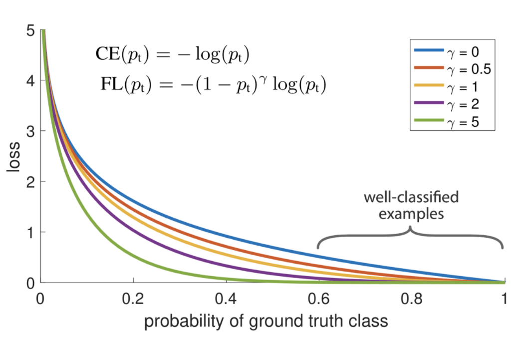
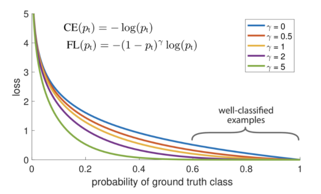
• \[\text{Cross Entropy}(p_{t}) = -\log{(p_{t})} \tag{3}\]
• \[\text{Focal Loss} = -(1 - p_{t})^{\gamma}\log{(p_{t})} \tag{4}\]

• 위 그래프와 식은 Focal Loss를 나타냅니다. Focal Loss와 Cross Entropy의 식을 비교해 보면 기본적인 Cross Entropy Loss에 \((1 - p_{t})^{\gamma}\) term이 더 추가된 것을 확인할 수 있습니다. 기본적인 Cross Entropy는 \(\gamma\) 가 0일 때 입니다.
• 여기서 추가된 \((1 - p_{t})^{\gamma}\) 의 역할은 easy example에 사용되는 loss의 가중치를 줄이기 위함입니다.
• 예를 들어 다음과 같은 2가지 경우를 살펴보겠습니다. 첫번째는 Foreground 케이스이며 이 때, \(Y = 1\) 이라고 하며 \(p = 0.95\) 라고 가정하겠습니다. 두번째는 Background 케이스이며 이 때, \(Y = 0\) 이라고 하며 \(p = 0.05\) 라고 가정하겠습니다.

• \[\text{CE(Foreground)} = -\log{(0.95)} = 0.05 \tag{5}\]
• \[\text{CE(Background)} = -\log{(1 - 0.05)} = 0.05 \tag{6}\]

• 식 (5)의 Foreground 케이스를 살펴보면 Foreground인 객체에 대하여 높은 확률인 0.95로 잘 분류하였고 그 결과 Loss가 0.05로 작은 것을 알 수 있습니다.
• 이와 유사하게 식 (6)의 Background 케이스를 살펴보면 Background임에 따라 낮은 확률인 0.05로 잘 분류하였고 그 결과 Loss가 0.05로 작은 것을 알 수 있습니다.
• 문제가 없어보이지만 여기서 발생하는 문제점은 Foregound 케이스와 Background 케이스 모두 같은 Loss 값을 가진다는 것에 있습니다. 왜냐하면 Background 케이스의 수가 훨씬 더 많기 때문에 같은 비율로 Loss 값이 업데이트되면 Background에 대하여 학습이 훨씬 많이 될 것이고 이 작업이 계속 누적되면 Foreground에 대한 학습량이 현저히 줄어들기 때문입니다.

Balanced Cross Entropy Loss의 한계

• Cross Entropy 케이스에서 발생하는 문제인 Foreground와 Background 케이스의 비율이 다른 점을 개선하기 위하여 Cross Entropy Loss 자체에 비율을 보상하기 위한 weight를 추가로 곱해주는 방법을 사용할 수 있습니다.
• 예를 들어 Foreground 객체의 클래스 수와 Background 객체의 클래스 수 각각의 역수의 갯수를 각 Loss에 곱한다면 클래스 수가 많은 Background의 경우 Loss가 작게 반영될 것이고 클래스 수가 적은 Foreground의 경우 Loss가 크게 반영될 것입니다.
• 이와 같이 각 클래스의 Loss 비율을 조절하는 weight \(w_{t}\) 를 곱해주어 imbalance class 문제에 대한 개선을 하고자 하는 방법이 Balanced Cross Entropy Loss 라고 합니다.
• 일반적으로 \(0 \le w_{t} \le 1\) 범위의 값을 사용하며 식으로 표현하면 다음과 같습니다.

• \[\text{CE}(p_{t}) = -w_{t}\log{(p_{t})} \tag{7}\]

• Cross Entropy Loss의 근본적인 문제가 Foreground 대비 Background의 객체가 굉장히 많이 나오는 class imbalance 문제에 해당하였습니다. 따라서 Balanced Cross Entropy Loss의 weight \(w\) 를 이용하면 \(w\) 에 대한 값의 조절을 통해 해결할 수 있을 것으로 보입니다. 즉, Forground의 weight는 크게 Background의 weight는 작게 적용하는 방향으로 개선하고자 하는 것입니다.
• 하지만 이와 같은 방법에는 문제점이 있습니다. 바로, Easy/Hard example 구분을 할 수 없다는 점입니다. 단순히 갯수가 많다고 Easy라고 판단하거나 Hard라고 판단하는 것에는 오차가 발생할 수 있습니다.
• 다음과 같은 예제를 살펴보겠습니다. 0.95의 확률로 Foreground 객체라고 분류한 Foreground 케이스에 weight 0.75를 주는 경우와 0.05의 확률로 Foreground 객체라고 분류 (즉, 0.95의 확률로 Background 객체라고 분류)한 Background 케이스에 weight 0.25를 주는 경우를 살펴보겠습니다.

• \[\text{CE(FG)} = -0.75 \log{(0.95)} = 0.038 \tag{8}\]
• \[\text{CE(BG)} = -(1 - 0.75) \log{(1 - 0.05)} = 0.0128 \tag{9}\]

• 앞에서 설명한 바와 같이 통상적으로 Background 객체의 수가 많으므로 더 낮은 Loss를 반영하기 위해 더 작은 weight를 반영하도록 하였습니다.
• 그리고 식을 살펴보면 Easy/Hard Example에 대한 반영은 전혀 없는 것 또한 알 수 있습니다.
• 따라서, Easy/Hard Example을 반영하기 위하여 이 글의 주제인 Focal Loss에 대하여 다루어 보도록 하겠습니다.

Focal Loss 알아보기

• Focal Loss는 Easy Example의 weight를 줄이고 Hard Negative Example에 대한 학습에 초점을 맞추는 Cross Entropy Loss 함수의 확장판이라고 말할 수 있습니다.
• Cross Entropy Loss 대비 Loss에 곱해지는 항인 \((1 - p_{t})^{\gamma}\) 에서 \(\gamma \ge 0\) 의 값을 잘 조절해야 좋은 성능을 얻을 수 있습니다.
• 추가적으로 전체적인 Loss 값을 조절하는 \(\alpha\) 값 또한 논문에서 사용되어 \(\alpha, \gamma\) 값을 조절하여 어떤 값이 좋은 성능을 가졌는 지 보여주었습니다. 식은 아래와 같고 논문에서는 \(\alpha = 0.25, \gamma = 2\) 를 최종적으로 사용하였습니다.

• \[\text{FL(p_{t})} = -\alpha_{t}(1 - p_{t})^{\gamma} \log{(p_{t})} \tag{10}\]

• 위 식에서 Foreground에 대해서는 \(\alpha = 0.25\) 가 적용되면 Background에 대해서는 \(\alpha = 0.75\) 가 적용되도록 사용됩니다.

• 위 그래프는 \(\gamma\) 가 0 ~ 5 까지 변화할 때의 변화를 나타내며 \(\gamma = 0\) 일 때, Cross Entropy Loss와 같고 \(\gamma\) 가 커질수록 Easy Example에 대한 Loss가 크게 줄어들며 Easy Examle에 대한 범위도 더 커집니다.
• 위 그래프를 통하여 Focal Loss의 속성을 크게 3가지 분류할 수 있습니다.
• ① 잘못 분류되어 \(p_{t}\) 가 작아지게 되면 \((1 - p_{t})^{\gamma}\) 도 1에 가까워지고 \(\log{(p_{t})}\) 또한 커져서 Loss에 반영됩니다.
• ② \(p_{t}\) 가 1에 가까워지면 \((1 - p_{t})^{\gamma}\) 은 0에 가까워지고 Cross Entropy Loss와 동일하게 \(\log{(p_{t})}\) 값 또한 줄어들게 됩니다.
• ③ \((1 - p_{t})^{\gamma}\) 에서 \(\gamma\) 를 focusing parameter 라고 하며 Easy Example에 대한 Loss의 비중을 낮추는 역할을 합니다.

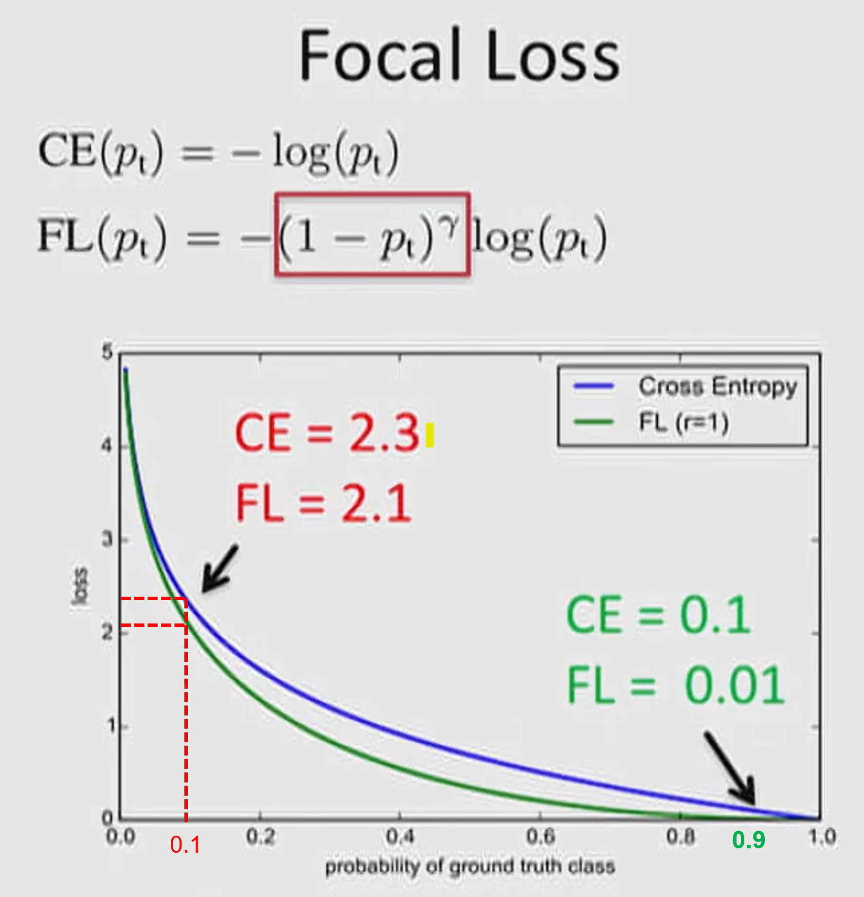
• 위 그림을 살펴보겠습니다. ① 빨간색 케이스의 경우 Hard 케이스의 문제이며 ② 초록색의 경우 Easy 케이스의 문제입니다. 그래프에 적용된 \(\alpha = 1, \gamma = 1\) 입니다.

• \[\text{CE}(p_{t}) = -\log{(p_{t})} \tag{10}\]
• \[\text{FL}(p_{t}) = -(1 - p_{t})\log{(p_{t})} \tag{11}\]

• ①에서는 \(p_{t} = 0.1\) 이므로 \(\text{CE}(0.1) = -\log{(0.1)} = 2.30259... \approx = 2.3\) 이고 \(\text{FL}(0.1) = -(1 - 0.1)\log{(0.1)} = 2.07233... \approx = 2.1\) 임을 알 수 있습니다.
• ②에서는 \(p_{t} = 0.9\) 이므로 \(\text{CE}(0.9) = -\log{(0.9)} = 0.105361... \approx = 0.1\) 이고 \(\text{FL}(0.9) = -(1 - 0.9)\log{(0.9)} = 0.0105361... \approx = 0.01\) 임을 알 수 있습니다.
• Hard 케이스 보다 Easy 케이스의 경우 weight가 더 많이 떨어짐을 통하여 기존에 문제가 되었던 수많은 Easy Negative 케이스에 의한 Loss가 누적되는 문제를 개선합니다.

• 지금까지 알아본 Focal Loss를 정리하면 다음과 같습니다.
• 배경(background)과 같은 Easy Negative 케이스는 딥러닝 모델의 정확도가 높기 때문에 loss는 작습니다. 하지만 Easy Negative 케이스의 갯수가 많아서 누적이 되면 전체 loss 값은 커지게 됩니다.
• 반면 실제 객체는 상대적으로 Hard 한 문제이고 따라서 loss 값은 커지지만 갯수가 작기 때문에 일반적으로 실제 객체 추정에 필요한 loss 의 총합보다 배경에 사옹된 loss의 총합이 커지는 문제가 발생한다.
• Focal loss는 Cross Entropy의 이러한 문제를 개선하고자 하며 Cross Entropy의 마지막에 출력되는 각 클래스의 probability에서 최종 확률값이 큰 Eays 케이스는 Loss를 크게 줄이고 최종 확률 값이 낮은 Hard 케이스는 Loss를 낮게 줄이는 역할을 합니다.
• 기본적으로 Cross Entropy는 확률이 낮은 케이스에 페널티를 주는 역할만 하고 확률이 높은 케이스에 어떠한 보상도 주지 않지만 Focal Loss는 확률이 높은 케이스에는 확률이 낮은 케이스 보다 Loss를 더 크게 낮추는 보상을 줍니다. 이 점이 차이점입니다.

Focal Loss Pytorch Code

• 아래 코드는 Focal Loss를 Semantic Segmentation에 적용하기 위한 Pytorch 코드입니다.
• Classification이나 Object Detection의 Task에 사용되는 Focal Loss 코드는 많으나 Semantic Segmentation에 정상적으로 동작하는 코드가 많이 없어서 아래와 같이 작성하였습니다.
• Cross Entropy Loss만 정확하게 짤 수 있다면 Cross Entropy Loss에 \((1 - p_{t})^{\gamma}\) 만 추가하면 되므로 어렵지 않습니다.

• \[\text{FL}(p_{t}) = -\alpha_{t}(1 - p_{t})^{\gamma}\log{(p_{t})} \tag{12}\]

• 지금부터 구현할 코드는 식 (12)를 사용할 수 있도록 구현합니다. 위 코드처럼 \(\alpha_{t}\) 을 추가하면 Balanced Cross Entropy 까지 적용할 수 있기 때문입니다.
• 아래 코드의 label_to_one_hot_label에서는 아래와 같은 원리로 \(\alpha_{t}\) 를 연산해 줍니다.

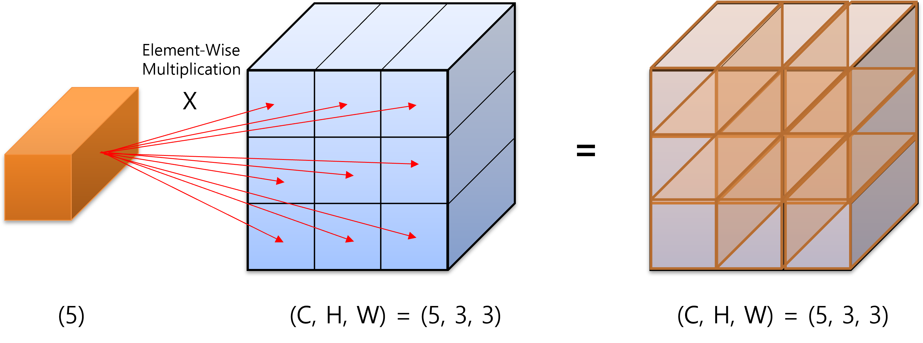
• 위 그림과 같이 클래스 별 weight를 담고 있는 one hot vector를 위 그림과 같이 연산을 합니다.

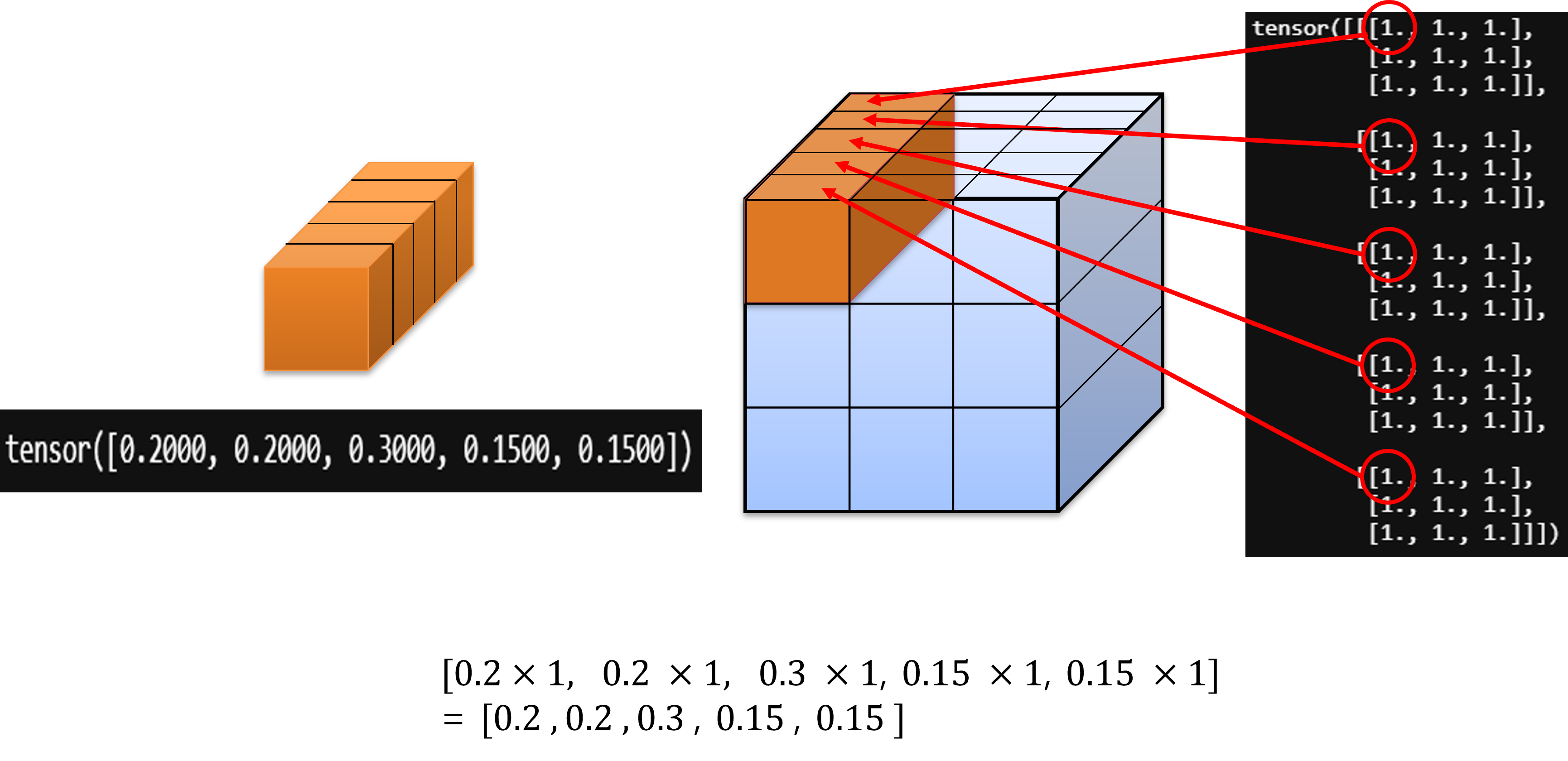
• 그러면 위 그림과 같이 channel 방향으로 주황색 one hot vector인 \(\alpha_{t}\) 가 최종 출력 (위 그림에서 모두 1로 되어 있는 tensor)에 곱해지게 됩니다.
• 또한 ignore label 기능을 지하기 위해 torch.split를 이용하여 필요하지 않는 인덱스를 삭제하도록 하였습니다.

import torch
import torch.nn as nn
import torch.nn.functional as F
import numpy as np
from typing import Optional

def label_to_one_hot_label(
    labels: torch.Tensor,
    num_classes: int,
    device: Optional[torch.device] = None,
    dtype: Optional[torch.dtype] = None,
    eps: float = 1e-6,
    ignore_index=255,
) -> torch.Tensor:
    r"""Convert an integer label x-D tensor to a one-hot (x+1)-D tensor.

    Args:
        labels: tensor with labels of shape :math:`(N, *)`, where N is batch size.
          Each value is an integer representing correct classification.
        num_classes: number of classes in labels.
        device: the desired device of returned tensor.
        dtype: the desired data type of returned tensor.

    Returns:
        the labels in one hot tensor of shape :math:`(N, C, *)`,

    Examples:
        >>> labels = torch.LongTensor([
                [[0, 1], 
                [2, 0]]
            ])
        >>> one_hot(labels, num_classes=3)
        tensor([[[[1.0000e+00, 1.0000e-06],
                  [1.0000e-06, 1.0000e+00]],
        
                 [[1.0000e-06, 1.0000e+00],
                  [1.0000e-06, 1.0000e-06]],
        
                 [[1.0000e-06, 1.0000e-06],
                  [1.0000e+00, 1.0000e-06]]]])

    """
    shape = labels.shape
    # one hot : (B, C=ignore_index+1, H, W)
    one_hot = torch.zeros((shape[0], ignore_index+1) + shape[1:], device=device, dtype=dtype)
    
    # labels : (B, H, W)
    # labels.unsqueeze(1) : (B, C=1, H, W)
    # one_hot : (B, C=ignore_index+1, H, W)
    one_hot = one_hot.scatter_(1, labels.unsqueeze(1), 1.0) + eps
    
    # ret : (B, C=num_classes, H, W)
    ret = torch.split(one_hot, [num_classes, ignore_index+1-num_classes], dim=1)[0]
    
    return ret


# https://github.com/zhezh/focalloss/blob/master/focalloss.py
def focal_loss(input, target, alpha, gamma, reduction, eps, ignore_index):
    
    r"""Criterion that computes Focal loss.

    According to :cite:`lin2018focal`, the Focal loss is computed as follows:

    .. math::

        \text{FL}(p_t) = -\alpha_t (1 - p_t)^{\gamma} \, \text{log}(p_t)

    Where:
       - :math:`p_t` is the model's estimated probability for each class.

    Args:
        input: logits tensor with shape :math:`(N, C, *)` where C = number of classes.
        target: labels tensor with shape :math:`(N, *)` where each value is :math:`0 ≤ targets[i] ≤ C−1`.
        alpha: Weighting factor :math:`\alpha \in [0, 1]`.
        gamma: Focusing parameter :math:`\gamma >= 0`.
        reduction: Specifies the reduction to apply to the
          output: ``'none'`` | ``'mean'`` | ``'sum'``. ``'none'``: no reduction
          will be applied, ``'mean'``: the sum of the output will be divided by
          the number of elements in the output, ``'sum'``: the output will be
          summed.
        eps: Scalar to enforce numerical stabiliy.

    Return:
        the computed loss.

    Example:
        >>> N = 5  # num_classes
        >>> input = torch.randn(1, N, 3, 5, requires_grad=True)
        >>> target = torch.empty(1, 3, 5, dtype=torch.long).random_(N)
        >>> output = focal_loss(input, target, alpha=0.5, gamma=2.0, reduction='mean')
        >>> output.backward()
    """
    if not isinstance(input, torch.Tensor):
        raise TypeError(f"Input type is not a torch.Tensor. Got {type(input)}")

    if not len(input.shape) >= 2:
        raise ValueError(f"Invalid input shape, we expect BxCx*. Got: {input.shape}")

    if input.size(0) != target.size(0):
        raise ValueError(f'Expected input batch_size ({input.size(0)}) to match target batch_size ({target.size(0)}).')

    # input : (B, C, H, W)
    n = input.size(0) # B
    
    # out_sie : (B, H, W)
    out_size = (n,) + input.size()[2:]
    
    # input : (B, C, H, W)
    # target : (B, H, W)
    if target.size()[1:] != input.size()[2:]:
        raise ValueError(f'Expected target size {out_size}, got {target.size()}')

    if not input.device == target.device:
        raise ValueError(f"input and target must be in the same device. Got: {input.device} and {target.device}")
    
    if isinstance(alpha, float):
        pass
    elif isinstance(alpha, np.ndarray):
        alpha = torch.from_numpy(alpha)
        # alpha : (B, C, H, W)
        alpha = alpha.view(-1, len(alpha), 1, 1).expand_as(input)
    elif isinstance(alpha, torch.Tensor):
        # alpha : (B, C, H, W)
        alpha = alpha.view(-1, len(alpha), 1, 1).expand_as(input)       
        

    # compute softmax over the classes axis
    # input_soft : (B, C, H, W)
    input_soft = F.softmax(input, dim=1) + eps
    
    # create the labels one hot tensor
    # target_one_hot : (B, C, H, W)
    target_one_hot = label_to_one_hot_label(target.long(), num_classes=input.shape[1], device=input.device, dtype=input.dtype, ignore_index=ignore_index)

    # compute the actual focal loss
    weight = torch.pow(1.0 - input_soft, gamma)
    
    # alpha, weight, input_soft : (B, C, H, W)
    # focal : (B, C, H, W)
    focal = -alpha * weight * torch.log(input_soft)
    
    # loss_tmp : (B, H, W)
    loss_tmp = torch.sum(target_one_hot * focal, dim=1)

    if reduction == 'none':
        # loss : (B, H, W)
        loss = loss_tmp
    elif reduction == 'mean':
        # loss : scalar
        loss = torch.mean(loss_tmp)
    elif reduction == 'sum':
        # loss : scalar
        loss = torch.sum(loss_tmp)
    else:
        raise NotImplementedError(f"Invalid reduction mode: {reduction}")
    return loss


class FocalLoss(nn.Module):
    r"""Criterion that computes Focal loss.

    According to :cite:`lin2018focal`, the Focal loss is computed as follows:

    .. math:

        FL(p_t) = -alpha_t(1 - p_t)^{gamma}, log(p_t)

    Where:
       - :math:`p_t` is the model's estimated probability for each class.

    Args:
        alpha: Weighting factor :math:`\alpha \in [0, 1]`.
        gamma: Focusing parameter :math:`\gamma >= 0`.
        reduction: Specifies the reduction to apply to the
          output: ``'none'`` | ``'mean'`` | ``'sum'``. ``'none'``: no reduction
          will be applied, ``'mean'``: the sum of the output will be divided by
          the number of elements in the output, ``'sum'``: the output will be
          summed.
        eps: Scalar to enforce numerical stabiliy.

    Shape:
        - Input: :math:`(N, C, *)` where C = number of classes.
        - Target: :math:`(N, *)` where each value is
          :math:`0 ≤ targets[i] ≤ C−1`.

    Example:
        >>> N = 5  # num_classes
        >>> kwargs = {"alpha": 0.5, "gamma": 2.0, "reduction": 'mean'}
        >>> criterion = FocalLoss(**kwargs)
        >>> input = torch.randn(1, N, 3, 5, requires_grad=True)
        >>> target = torch.empty(1, 3, 5, dtype=torch.long).random_(N)
        >>> output = criterion(input, target)
        >>> output.backward()
    """

    def __init__(self, alpha, gamma = 2.0, reduction = 'mean', eps = 1e-8, ignore_index=30):
        super().__init__()
        self.alpha = alpha
        self.gamma = gamma
        self.reduction = reduction
        self.eps = eps
        self.ignore_index = ignore_index

    def forward(self, input, target):
        return focal_loss(input, target, self.alpha, self.gamma, self.reduction, self.eps, self.ignore_index)

deep learning 관련 글 목차