(멀티플 뷰 지오메트리) Lecture 4. Robust homography estimation

2022, Apr 20    

Multiple View Geometry 글 목차

• 참조 : https://youtu.be/W8vgVoQdwAM?list=PLxg0CGqViygP47ERvqHw_v7FVnUovJeaz
• 참조 : https://youtu.be/v3322cNhCTk?list=PLxg0CGqViygP47ERvqHw_v7FVnUovJeaz
• 참조 : Multiple View Geometry in Computer Vision

• 이번 강의를 이해하기 위해 아래 사전 지식이 필요합니다.
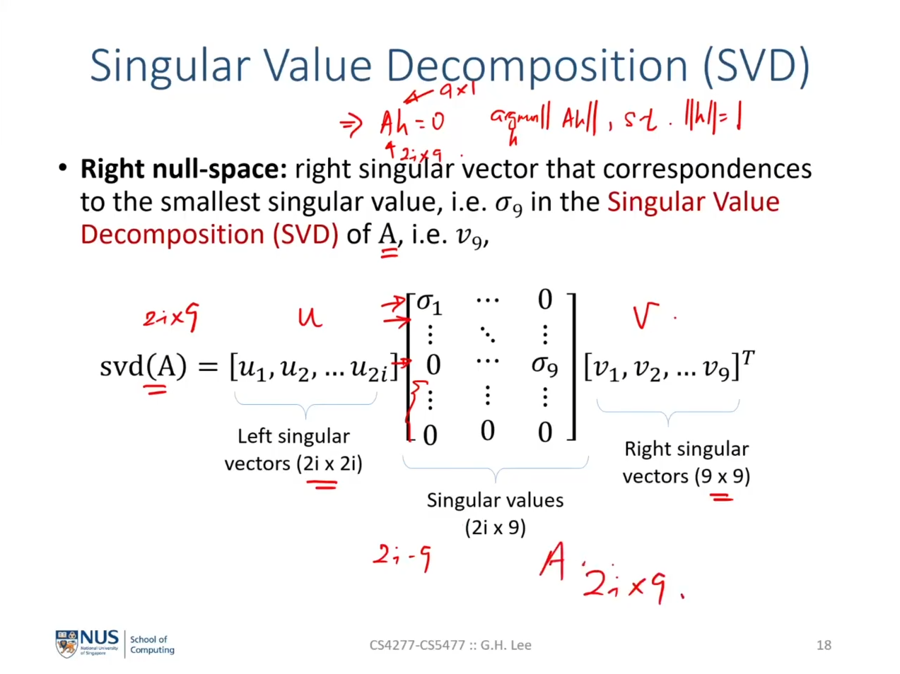
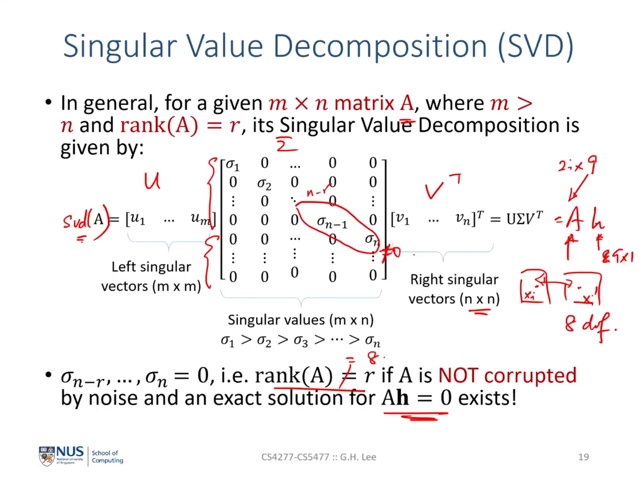
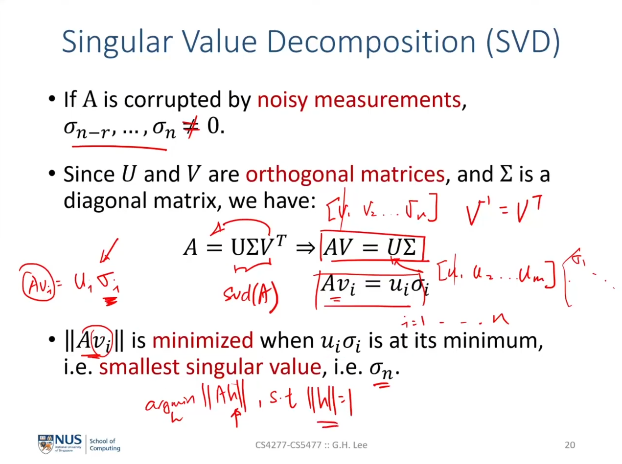
• least squrares : https://gaussian37.github.io/math-la-least_squares/
• rank : https://gaussian37.github.io/math-la-rank/
• SVD (Singular Value Decomposition) : https://gaussian37.github.io/math-la-svd/

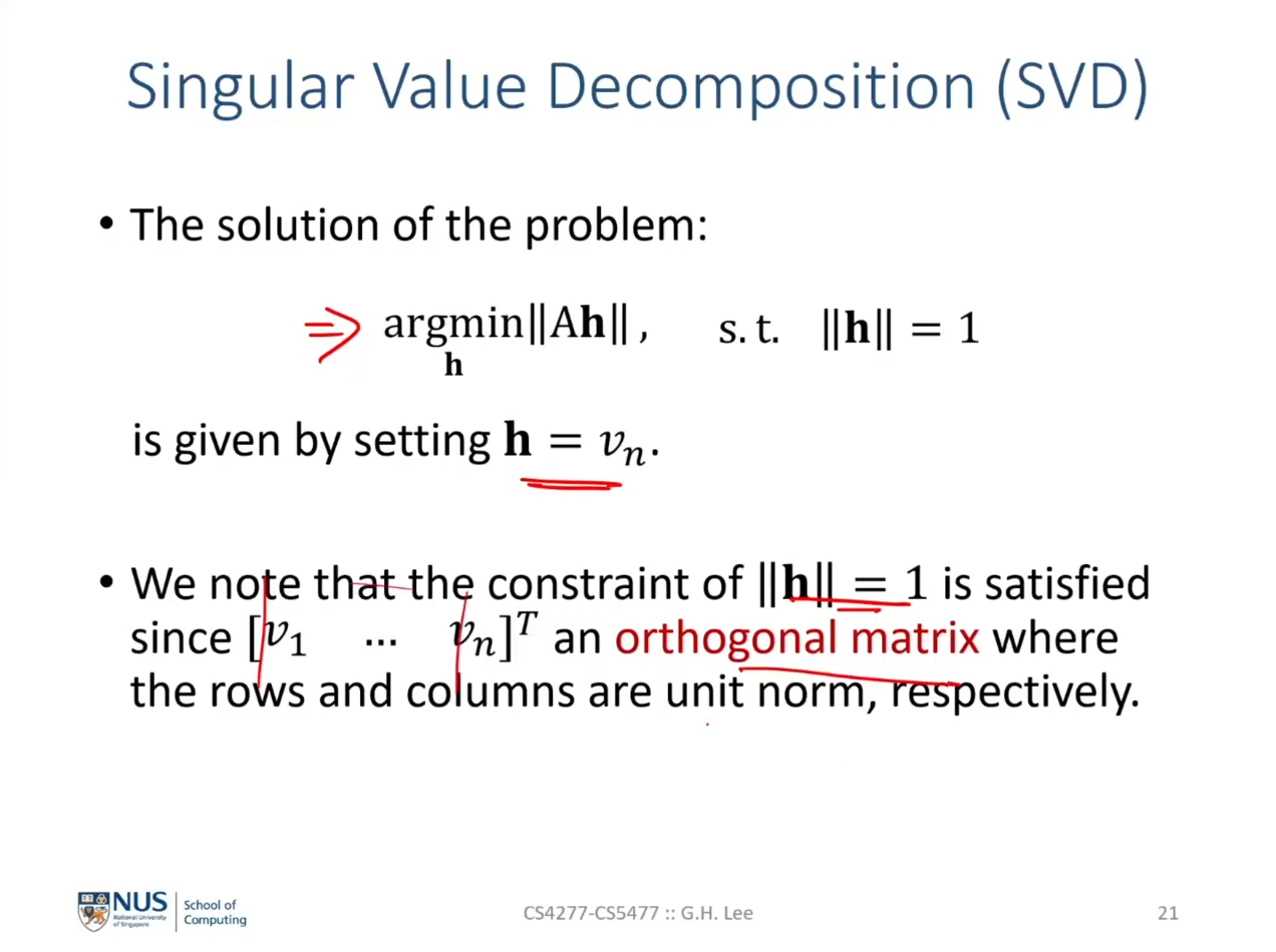
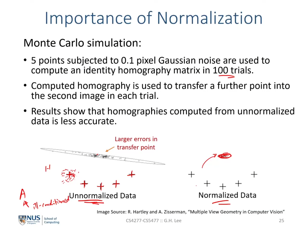
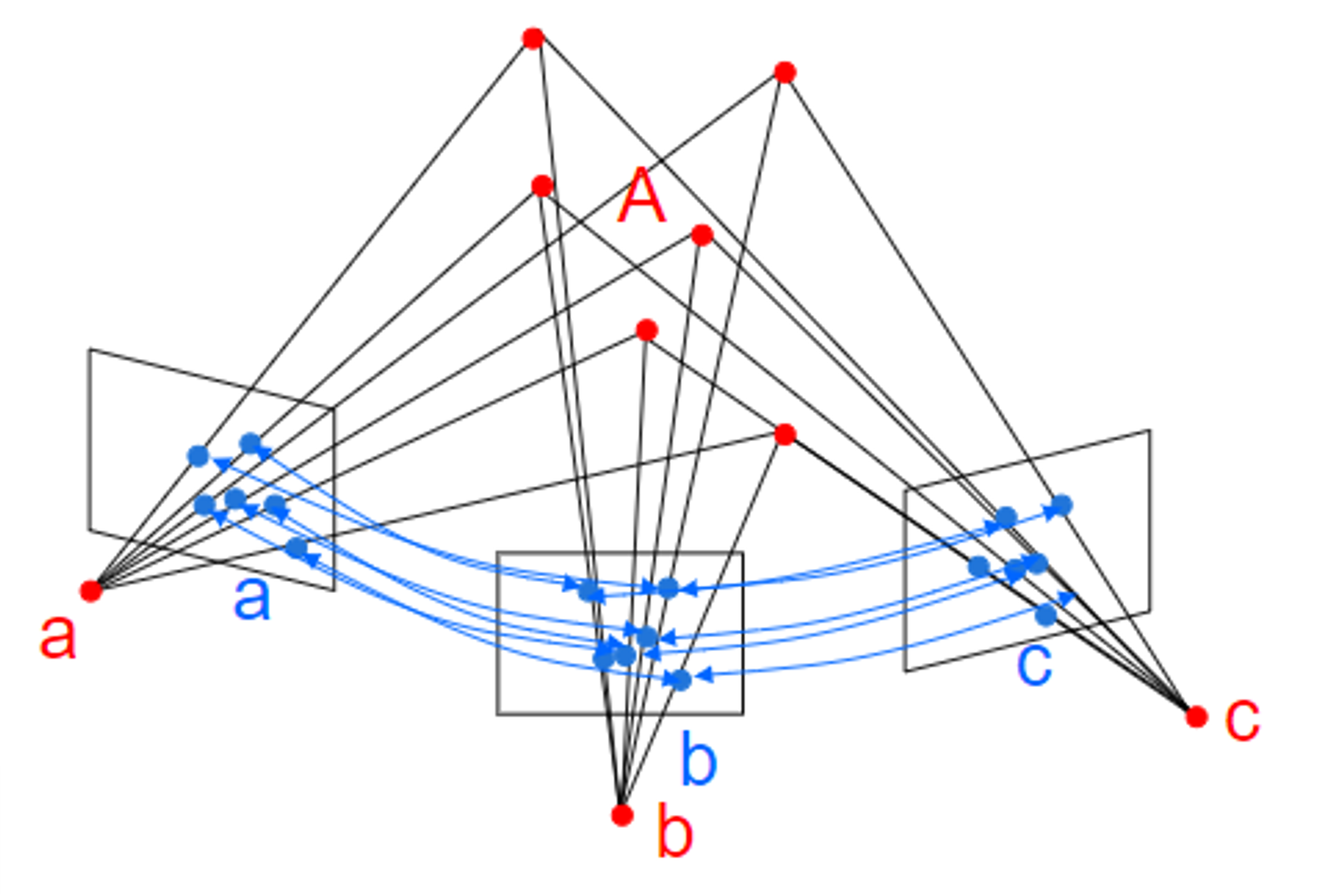
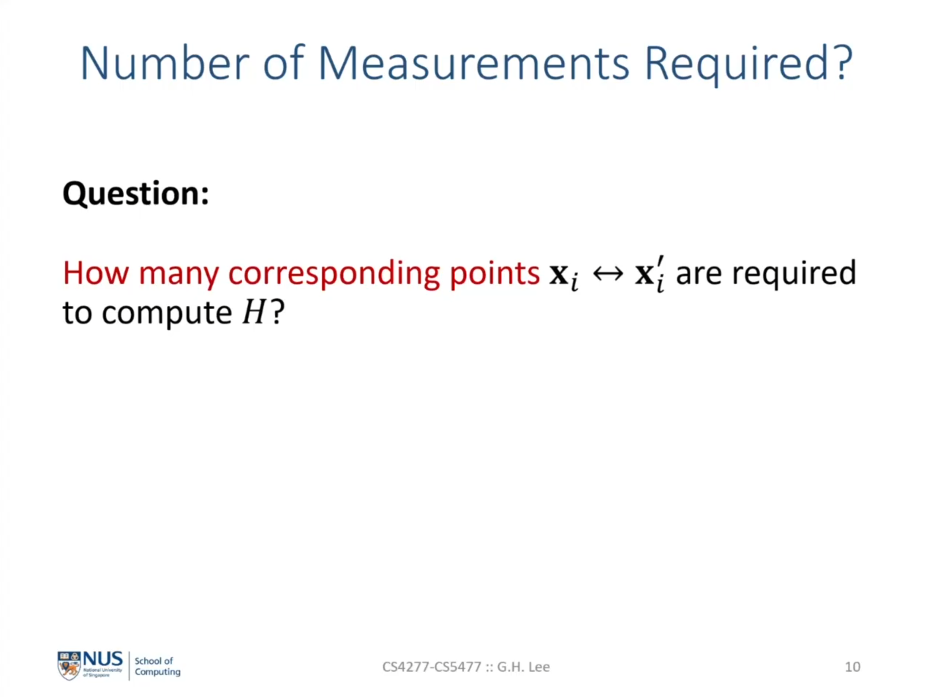
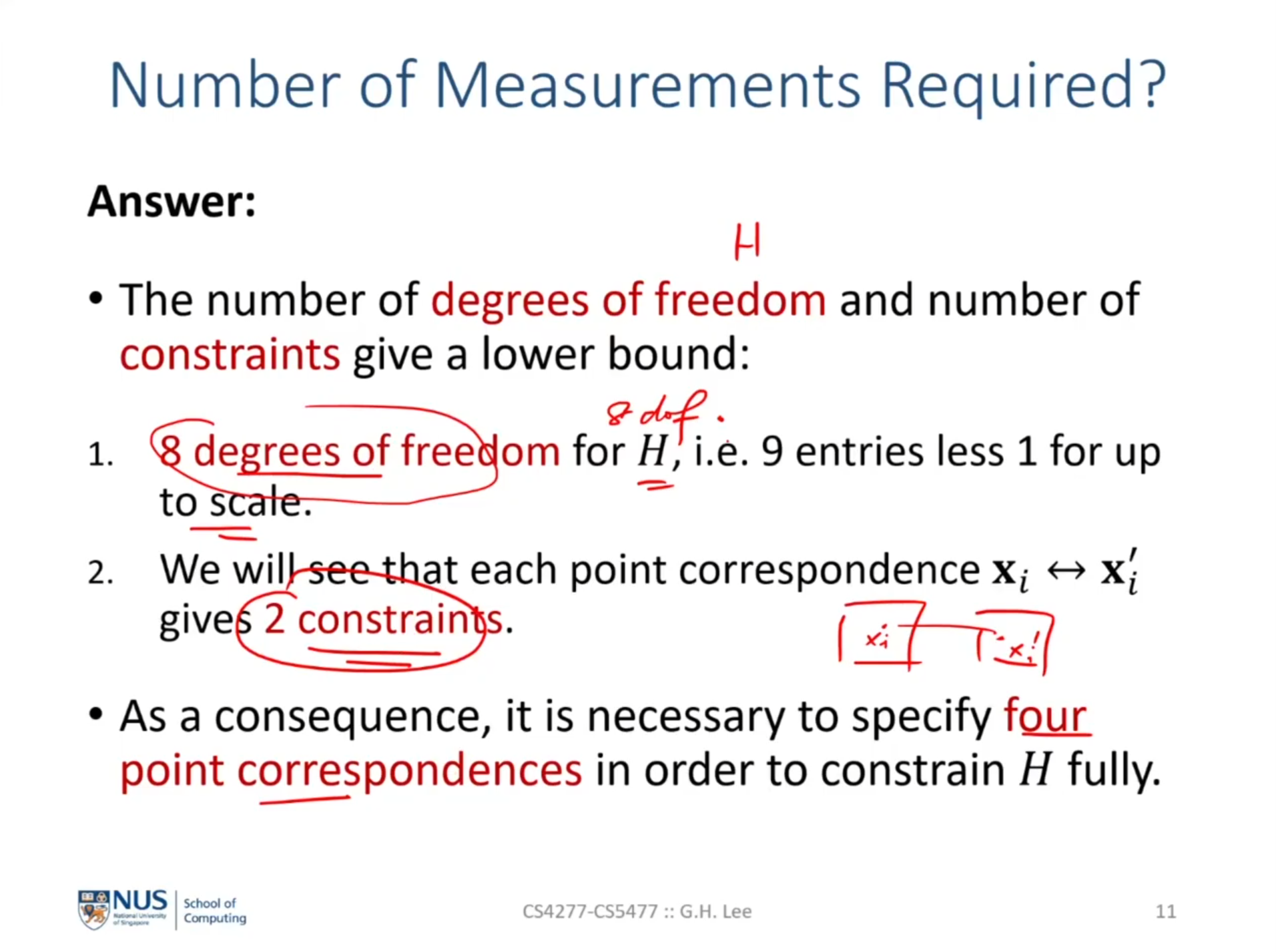
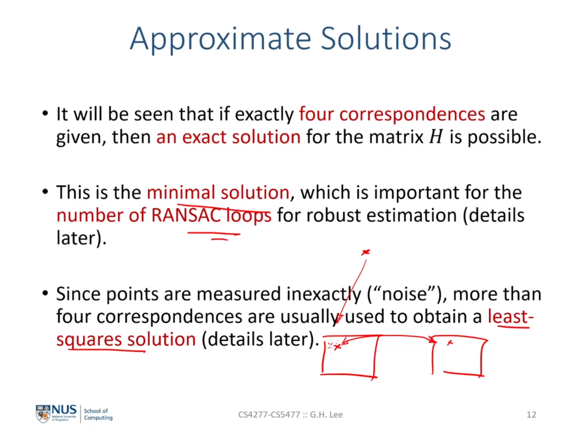
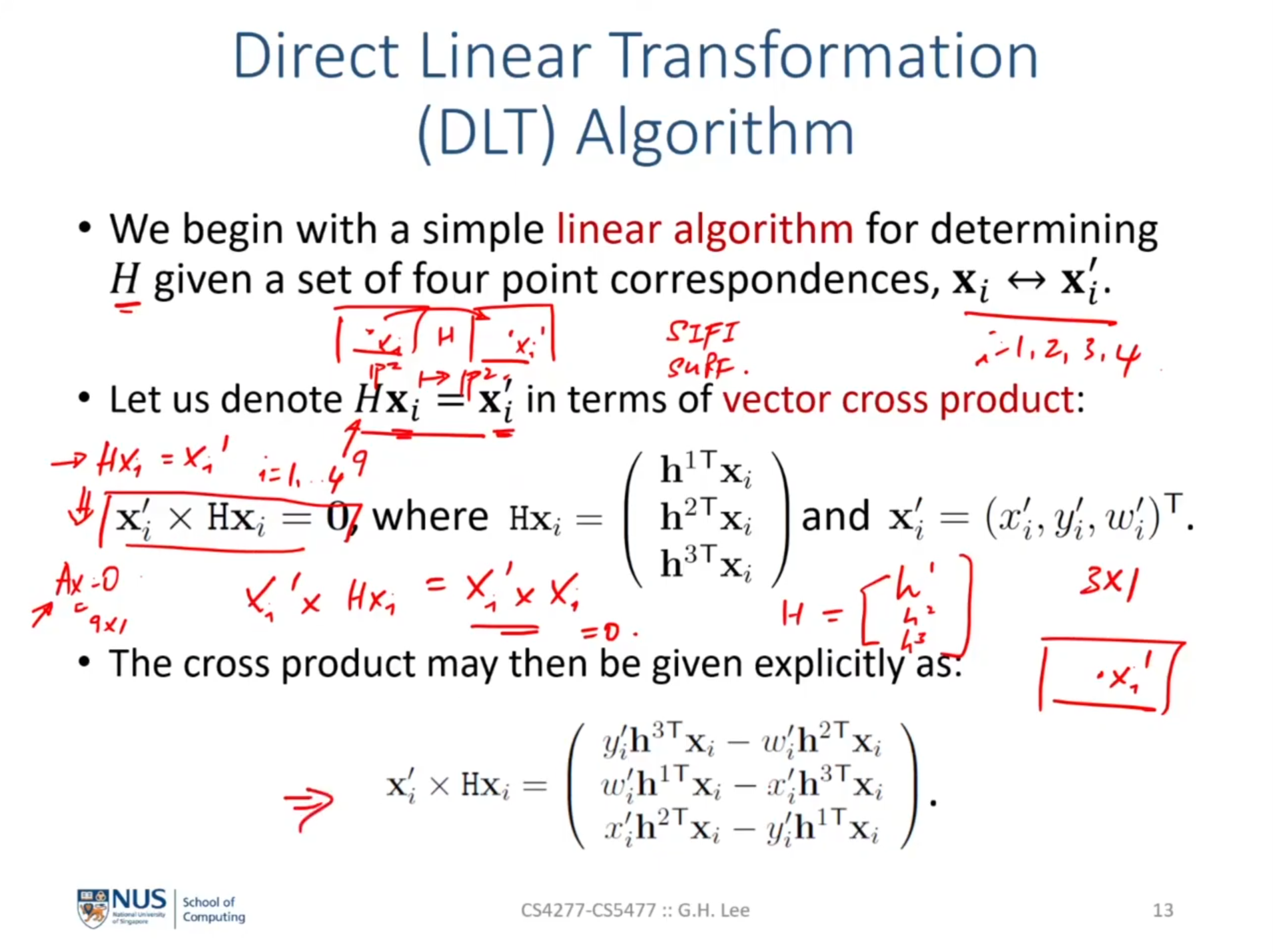
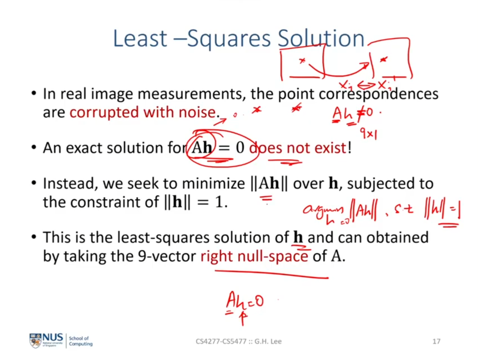
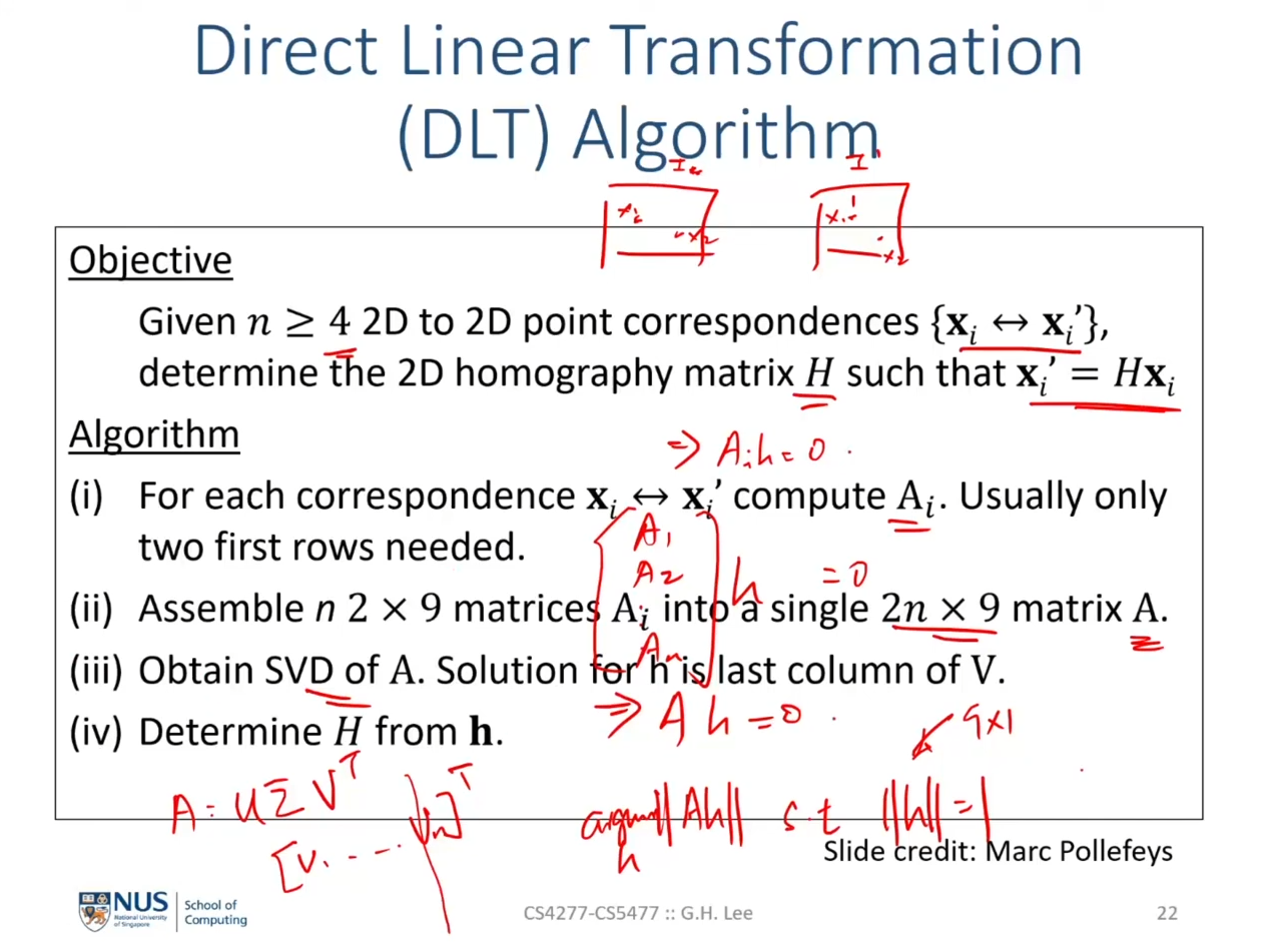
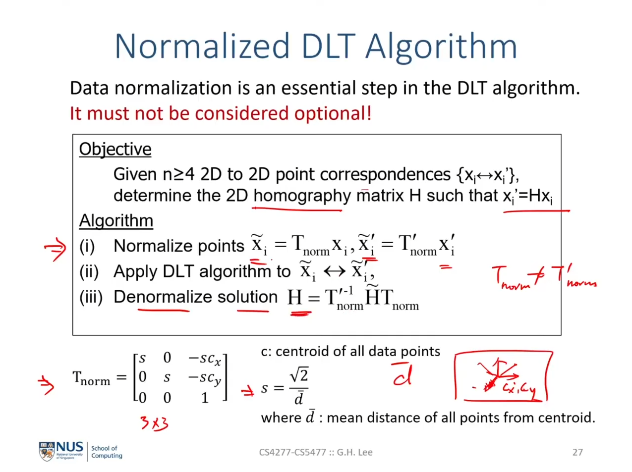
• 안정적인 DLT 알고리즘을 구현하기 위하여 Nomalied DLT 알고리즘을 필수적으로 사용하기를 권장하며 전체적인 알고리즘의 순서는 위 표와 같습니다.
• 4개 이상의 2D 포인트 간의 대응 $x_{i} \leftrightarrow x_{i}'$ 이 주어지면 2D homography 행렬 $H$ 를 구할 수 있으며 구 역할은 $x_{i}' = H x_{i}$ 와 같습니다.

• normalized DLT 알고리즘은 다음과 같습니다.

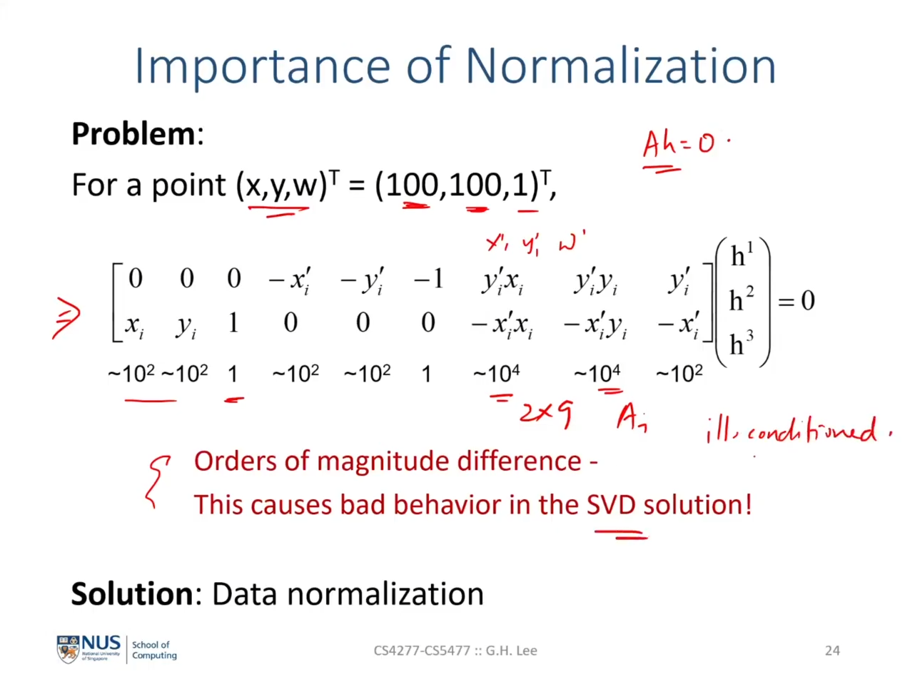
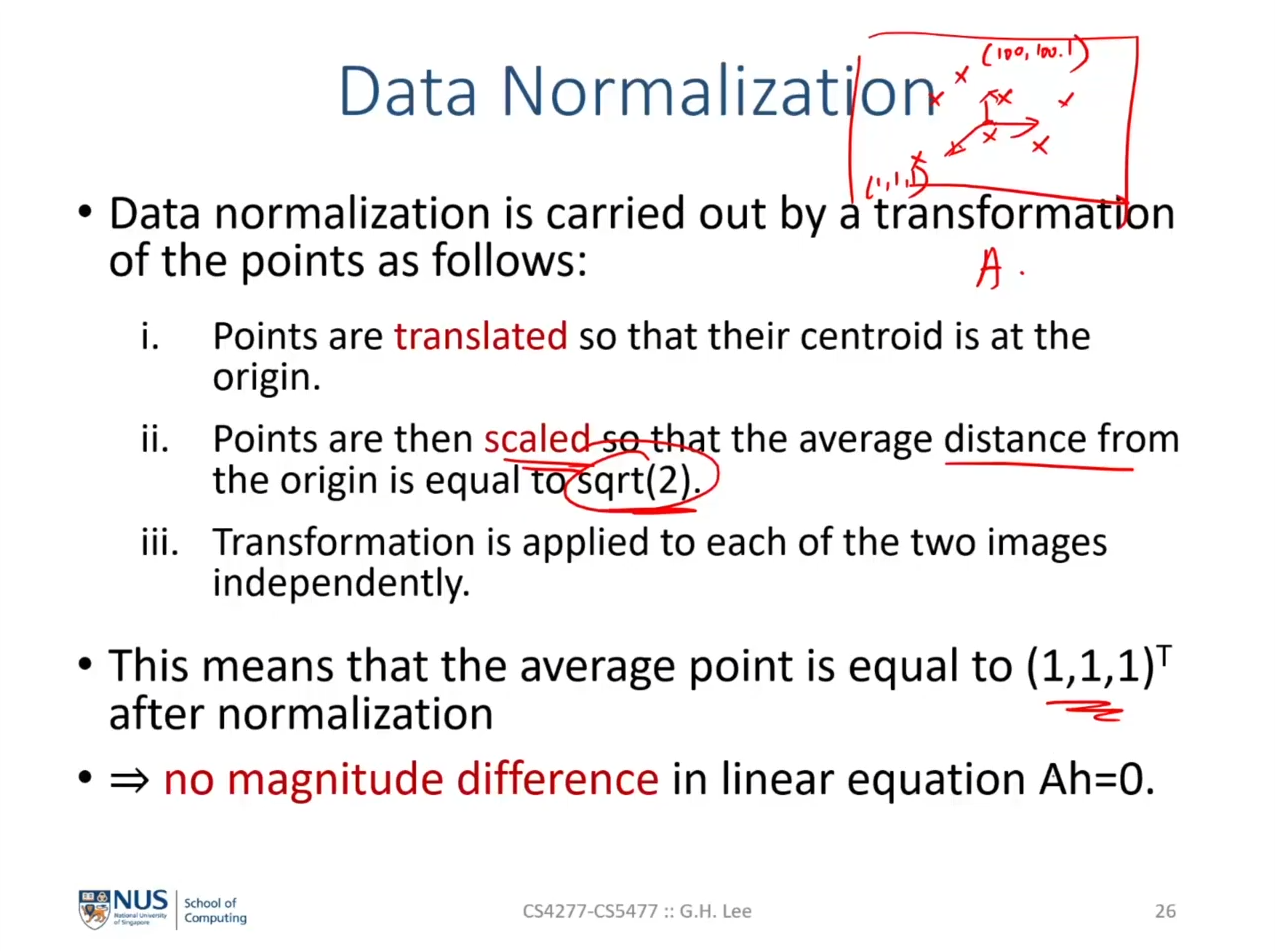
• ① 각 대응된 포인트 $x_{i} \leftrightarrow x_{i}'$ 를 $T_{\text{norm}}$ 과 $T_{\text{norm}}'$ 각각을 이용하여 normalize를 적용합니다. $T_{\text{norm}}$ 은 $x_{i}$ 를 normalize 하는 변환 행렬이며 $T_{\text{norm}}'$ 는 $x_{i}'$ 를 normalize 합니다. 즉, 각 2D image coordinate에서 각 포인트 값에 맞게 normalize 하게 됩니다. 변환 행렬은 다음과 같이 구성됩니다.

• $$T_{\text{norm}} = \begin{bmatrix} s & 0 & -s c_{x} \\ 0 & s & -s c_{y} \\ 0 & 0 & 1 \end{bmatrix}$$
• $$c = (c_{x}, c_{y}) = \text{centroid of all data points}$$
• $$s = \frac{\sqrt{2}}{\bar{d}}$$
• $$\bar{d} = \text{mean distance of all points from centroid}$$

• 위 식에서 $s$ 는 평균 distance 를 $sqrt{2} = \sqrt{ (1 - 0)^{2} + (1 - 0)^{2} }$ 에 나눔으로써 $x, y$ 방향으로 거리가 1이고 원점으로 부터 distance가 $sqrt{2}$ 인 공간으로 normalization 하는 scale 값으로 사용 되었습니다.
• 따라서 $T_{\text{norm}}$ 를 이용하여 scale 변화와 centroid 까지의 이동 까지 반영하여 normalize 할 수 있습니다.

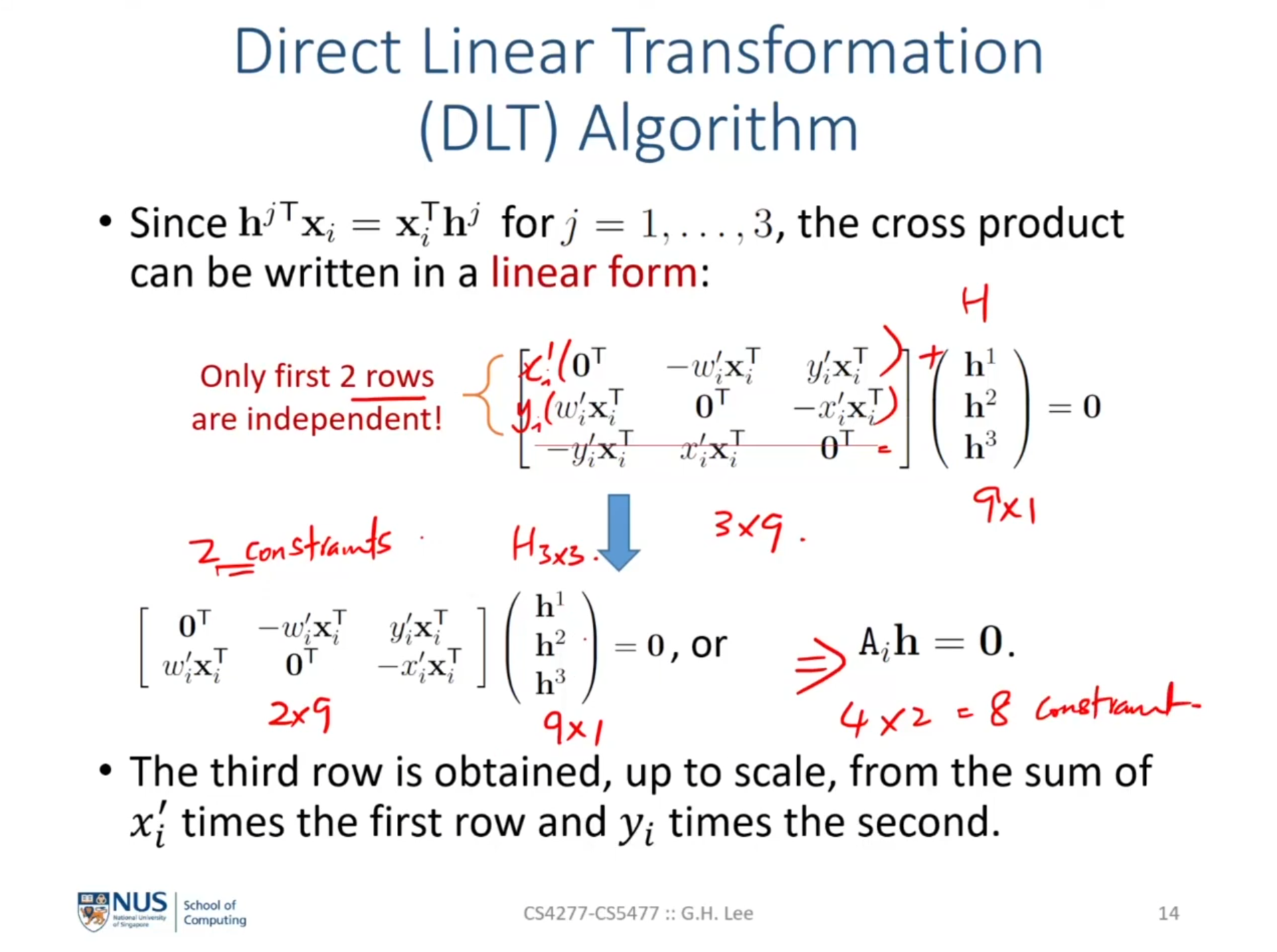
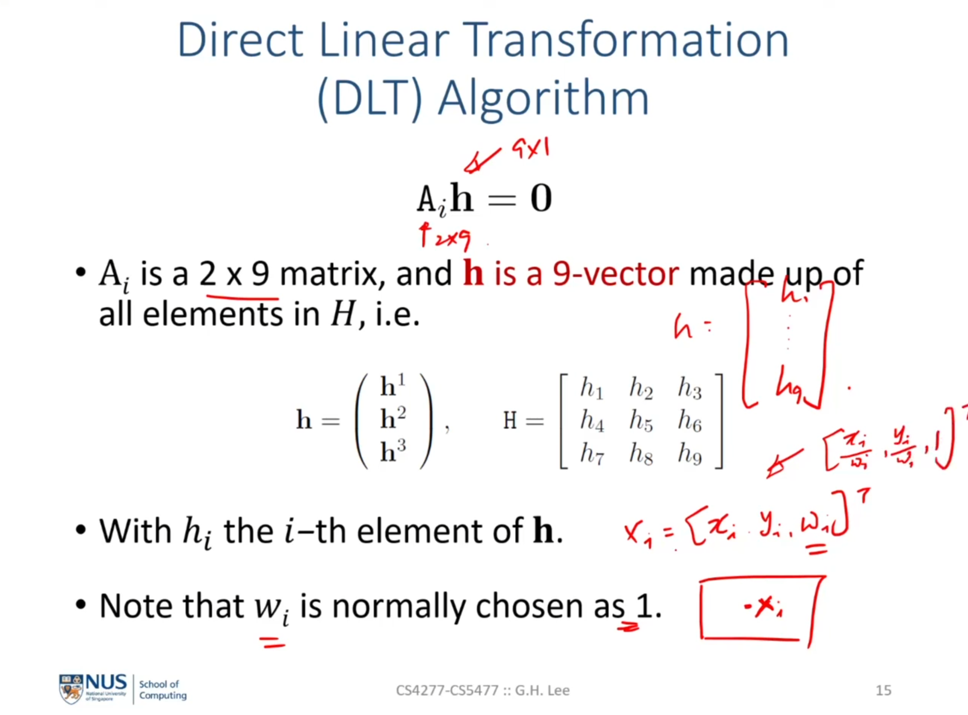
• ② 앞에서 다룬 방식과 동일하게 DLT 알고리즘을 사용하여 $\tilde{x}_{i} \leftrightarrow \tilde{x}_{i}'$ 간 변환을 하는 homography $\tilde{H}$ 를 구할 수 있습니다. normalize된 공간에서의 homography이기 때문에 $\tilde{H}$ 로 표현합니다.

• ③ 실제 사용해야 하는 homography는 image coordinate의 homography인 $H$ 이므로 다음과 같이 구할 수 있습니다.

• $$H = T_{\text{norm}}'^{-1} \tilde{H} T_{\text{norm}}$$
• $$T_{\text{norm}} : \text{image space} \to \text{normalized space}$$
• $$\tilde{H} : \text{normalized space homography}$$
• $$T_{\text{norm}}'^{-1} : \text{normalized space} \to \text{image space}$$

• 따라서 $H$ 는 image space에서 적용하는 homography가 되며 그 내부 과정을 살펴보면 image space → normalized space → normalized space homography → image space 순서로 변환 과정이 누적됩니다.

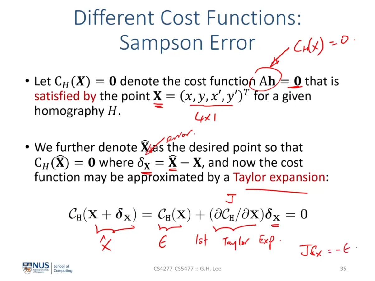
• 어떤 함수 $f(x)$ 를 테일러 급수로 근사화 하면 다음과 같이 나타낼 수 있습니다. 아래 $p_{n}(x)$ 가 $n$ 차항 까지 근사화 한 것이고 $n \to \infty$ 가 되면 $f(x) = p_{\infty}(x)$ 를 만족하는 것이 테일러 급수의 성질입니다.

• $$f(x) = p_{\infty}(x)$$
• $$\begin{align} f(x) &= p_{n}(x) = f(a) + f'(a)(x - a) + \frac{f''(a)}{2!}(x-a)^{2} + \cdots + \frac{f^{n}(a)}{n!}(x-a)^{n} \\ &= \sum_{k=0}^{n} \frac{f^{k}(a)}{k!}(x-a)^{k} \end{align}$$

• 테일러 급수를 변화량 $h$ 와 함께 표현하면 다음과 같이 나타낼 수 있으며 위 식과 표현에 차이만 있을 뿐 의미는 같습니다.

• $$\begin{align} f(a + h) &= f(a) + f'(a)h + \frac{f^{2}(a)}{2!}h^{2} + \frac{f^{3}(a)}{3!}h^{3} + \cdots + \frac{f^{n}(a)}{n!}h^{n} \\ &= \sum_{k=0}^{n} \frac{f^{k}(a)}{k!}h^{k} \end{align}$$

Multiple View Geometry 글 목차