CGNet, A Light-weight Context Guided Network for Semantic Segmentation
2019, Nov 05
- 논문 : https://arxiv.org/abs/1811.08201
- 코드 : https://github.com/wutianyiRosun/CGNet
- Cityscape Benchmarks 성능 : ① IoU class : 64.8 %, ② Runtime : 20 ms
- 링크 : https://www.cityscapes-dataset.com/method-details/?submissionID=2095
- 이번 글에서는 CGNet, A Light-weight Context Guided Network for Semantic Segmentation 에 대하여 알아보도록 하겠습니다.
- Network의 이름에도 포함이 되어 있듯이
Light-weight이므로 weight의 수가 작은 Realtime 용도의 Segmentation 모델입니다.
목차
-
Abstract
-
Introduction
-
Related Work
-
Proposed Approach
-
Experiments
-
Pytorch code
Abstract
- 세그멘테이션(semantic segmentation)을 모바일 디바이스 환경에 적용하려는 시도가 많이 증가하고 있습니다.
- 성능이 좋은 세그멘테이션 모델들은 많은 파라미터와 연산량으로 인해 모바일 디바이스에는 적합하지 않기 때문에 모바일 디바이스에는 경량화 모델이 필요합니다.
- 경량화 세그멘테이션 모델에 대한 연구들의 일부 문제점은 classification에서 사용된 방법들을 사용하고 세그멘테이션에서 고려해야 할 특성들을 무시한 상태로 구조가 만들어 졌다는 것에 있습니다.
- 이 논문에서는 이러한 문제점들을 개선하기 위하여
Context Guided Network (CGNet)을 소개합니다. 이 모델 또한 가볍고 계산에 효율적인 세그멘테이션 모델입니다. - CGNet에서 사용된
CG block은 local feature와 local feature를 둘러싼 surrounding context를 학습합니다. 그리고 더 나아가 global context와 관련된 feature 또한 이용하여 성능을 향상시킵니다. CGNet은CG block을 기반으로 네트워크의 모든 단계에서 상황에 맞는 정보를 이해하고 세그멘테이션 정확도를 높이기 위해 설계됩니다. (local feature는 convolutional filter가 연산되는 영역입니다.) - CGNet은 또한 파라미터 수를 줄이고 메모리 공간을 절약하도록 정교하게 설계되었습니다. 동등한 수의 매개 변수 하에서 제안된 CGNet은 기존 세그먼테이션 네트워크보다 훨씬 뛰어납니다.
- Cityscape 및 CamVid 데이터 세트에 대한 광범위한 실험은 제안된 접근 방식의 효과를 검증합니다.
- 특히 post-processing 및 multi-scale testing 없이 제안 된 CGNet은 0.5M 미만의 매개 변수로 64.8 %의 Cityscape에서 평균 IoU를 달성합니다.
Introduction
- 최근 자율주행 및 로봇 시스템에 대한 관심이 높아지면서 모바일 장치에 세그멘테이션 모델을 배치해야 한다는 요구가 거세지고 있습니다. 하지만 작은 메모리을 사용하면서 높은 정확도를 모두 갖춘 모델을 설계하는 것은 중요하고 어려운 일입니다.
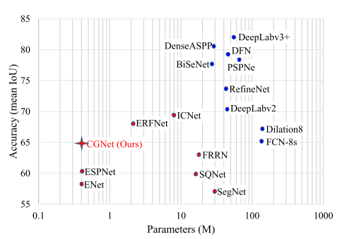
- 위 그림은 Cityscape 데이터 셋에서 여러 가지 모델의 정확도와 매개변수 수를 보여줍니다. 그래프의 파란색 점은 정확도가 높은 모델을 나타내고 빨간색 점은 메모리 사용량이 작은 모델을 나타냅니다.
CGNet은 메모리 사용량이 작은 방법에 비해 파라미터 수가 적으면서도 정확도가 높아 왼쪽 상단에 위치합니다. - 위 그래프의 파란색 점에 해당하는 모델들은 모바일 디바이스에서 사용하기 적합하지 않습니다.
- 반면 빨간색 점들은 이미지 분류의 설계 원리를 따를 뿐 세그멘테이션의 고유한 속성은 무시하기 때문에 세그멘테이션 정확도가 낮습니다.
- 따라서 CGNet은 정확성을 높이기 위해 세그멘테이션의 내재적 특성을 활용하는 방법으로 설계됩니다.
- 세그멘테이션은 픽셀 수준 분류와 개체 위치 지정을 모두 포함합니다. 따라서 공간 의존성(spatial dependency)과 상황별 정보(contextual information)는 정확성을 향상시키는 중요한 역할을 합니다.
- ①
CG 블록은 local feature와 주변 context가 결합된 joint feature를 학습합니다. 따라서 CG블록은 local feature와 local feature 주변의 context가 공간 상 공유하는 특징들을 잘 학습하게 됩니다. - ②
CG 블록은 global context를 사용하여 ①에서 만든 joint feature를 개선합니다. global context는 유용한 구성요소를 강조하고 쓸모 없는 구성요소를 억제하기 위해 채널별로 joint feature의 가중치를 재조정하는 데 적용됩니다. global context에 대한 상세 내용은 뒤에서 알아보겠습니다. - ③
CG 블록은 CGNet의 모든 단계에서 활용됩니다. 따라서, CCNet은 (깊은 레이어) semantic level 과 (얕은 레이어) spatial level 모두에서 context 정보를 캡처합니다. 이는 기존 이미지 분류 방법에 비해 세그멘테이션에 더 적합합니다.
- 기존 세그멘테이션 프레임워크는 두 가지 유형으로 나눌 수 있습니다.
- 앞에서 다룬 CGNet의 성과에 대하여 정리하면 다음과 같습니다.
- ① local feature와 local feature의 주변 context feature를 합친 joint feautre를 학습하고 global context로 joint feature를 더욱 향상시키는 CG 블록을 제안하여 세그멘테이션 성능을 높였습니다.
- ② CG 블록을 적용하여 모든 단계에서 context 정보를 효과적이고 효율적으로 캡처하는 CGNet을 설계하였습니다. 특히, CCNet의 backbone은 세그멘테이션 정확도를 높이기 위해 맞춤 제작되었습니다.
- ③ 파라미터 수와 메모리 사용량을 줄이기 위해 CCNet의 아키텍처를 정교하게 설계하였습니다. 동일한 수의 매개 변수에서 제안된 CGNet은 기존 세그멘테이션 네트워크(예: ENet 및 ESPNet)의 성능을 크게 능가합니다.
Related Work
- Related Work에서는 CGNet과 관련된 작은 세그멘테이션 모델(small semantic segmentation model), 상황별 정보(contextual information) 모델 그리고 어텐션 모델에 대하여 간략하게 다루어 보겠습니다.
Small semantic segmentation models
- 작은 세그멘테이션 모델을 사용하려면 정확성과 모델 매개변수 또는 메모리 공간 간에 적절한 trade-off가 필요합니다.
ENet은 FCN과 같은 기존 세그멘테이션 모델의 마지막 단계를 제거하는 방법을 제안하고 임베디드 장치에서 세그멘테이션이 가능하다는 것을 보여주었습니다.- 반면 그러나
ICNet은 compressed-PSPNet 기반 이미지 캐스케이드 네트워크를 제안하여 의미 분할 속도를 높였습니다. - 최근의
ESPNet에서는 리소스 제약 하에서 고해상도 이미지를 세그멘테이션할 수 있는 빠르고 효율적인 콘볼루션 네트워크를 도입했습니다. - 하지만
ENet,ICNet,ESPNet과 같은 모델 대부분은 영상 분류의 설계 원리를 따르기 때문에 픽셀 별 세그멘테이션 정확도가 떨어집니다.
Contextual information models
- 최근 연구에서는 상황별 정보가 고품질 세그멘테이션 결과를 예측하는 데 도움이 된다는 것을 보여 주었습니다.
- 한 가지 방법은 필터의 receptive field를 확대하거나 또는 상황에 맞는 정보를 캡처하도록 특정 모듈을 구성하는 것입니다.
- 예를 들어
dilation 8은 Class likelihood map 이후에 multiple dilated convolutional layers을 사용하여 exercise multi-scale context를 합칩니다. (aggregation) - 또는
SAC(scale-adaptive convolution)는 가변적인 크기의 receptive field를 적용합니다. DeepLab v3는 ASPP, Atrous Spatial Pyramid Pooling을 도입합니다. ASPP를 이용하여 상황별 정보를 다양한 크기(스케일)로 얻을 수 있습니다.
Attention models
- 최근, Attention 메커니즘은 모델의 능력 향상을 위해 널리 사용되고 있습니다. RNNsearch는 machine translation에서 target word를 예측할 때 input words에 가중치를 주는 방법을 제안합니다.
- 세그멘테이션 모델에도 Attenstion 메커니즘 기법들이 사용되고 있습니다.
CG 블록은 global context 정보를 사용하여 weight vector를 계산합니다. 이 정보는 local feature와 surrounding context feature의 joint feature를 개선하기 위해 사용됩니다.
Proposed Approach
- 지금 부터
CG block에 대하여 다루어 보고 CG block과 유사한 다른 구조의 block과 비교를 해보겠습니다.
Context Guided Block
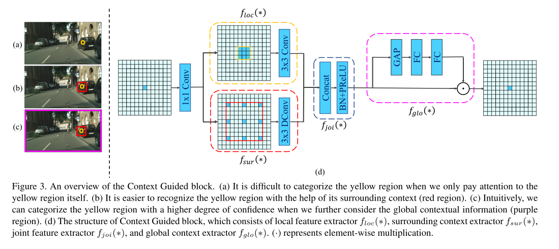
- 먼저 위 그림을 설명하고 Context Guided Block에 대하여 다루어 보도록 하겠습니다.
- 먼저 (a)를 보면 그림의 조그마한 노란색 영역만 보았을 때, 그 영역에 해당하는 클래스가 무엇인지 판단하기가 어렵습니다.
- 반면 (b)와 같이 노란색 영역 주위에 빨간색 영역을 포함하여 같이 본다면 인식하기 좋아집니다. 여기서 빨간색 영역을
surrounding context라고 합니다. - 마지막으로 (c) 그림을 보면 전체 이미지를 포함하는 보라색의 사각형이 있습니다. 전체 영역을 이용하여 노란색 영역의 클래스가 무엇인 지 판단한다면 더 높은 정확도로 판단할 수 있습니다. 보라색 사각형을
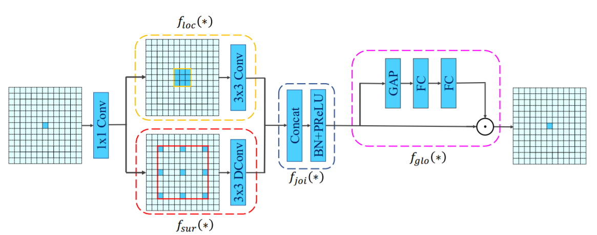
global context라고 하겠습니다. - CG 블록의 형태는 (d)와 같습니다. 블록의 구성 요소 중 \(f_{loc}(*)\) 이 그림의 노란색 영역에 해당하는 local feature입니다. 그리고 \(f_{sur}(*)\)은 빨간색 영역에 해당하는 surrounding context extractor 입니다. \(f_{joi}(*)\)는 \(f_{loc}(*)\)와 \(f_{sur}(*)\)을 합친 joint feature 입니다. 마지막으로 \(f_{glo}(*)\)는 global context extractor 입니다. 그림의 마지막에 있는 ⊙ 기호는 element-wise multiplication을 뜻합니다.
CG 블록은 인간 시각 시스템에서 영감을 얻었는데, 이것은 장면을 이해하기 위해 상황별 정보에 의존합니다.- 위 그림의 (a)와 같이 인간의 시각 시스템이 황색 영역을 인식하려 한다고 가정해 보겠습니다. 이 영역 자체에만 주의를 기울이면 판단하기 어려운 영역입니다. 추가적으로 (b)와 같이 빨간색 영역을 노란색 영역의 주변 컨텍스트로 정의해 보겠습니다.
- 노란색 영역과 주변 컨텍스트 즉, 상황을 모두 얻을 경우 더 쉽게 노란색 영역에서 픽셀 별 카테고리를 정할 수 있습니다. 따라서 주변 컨텍스트는 세그멘테이션에 유용합니다.
- 더 나아가서 (c)와 같이 황색 영역 및 주변 상황(빨간색 영역)과 함께 전체 장면의 전역 컨텍스트를 추가로 캡처할 경우 황색 영역을 분류할 수 있는 신뢰도가 더 높습니다. 따라서 주변 컨텍스트와 전역 컨텍스트는 모두 세그멘테이션 정확도를 높이는 데 유용합니다.
- 위의 분석을 바탕으로 CG 블록을 도입하여
local feature,surrounding context및global context를 최대한 활용합니다. - 앞에서 정의한 용어로 다시 살펴보면 다음과 같습니다.
- ① \(f_{loc}(*)\) : local feature (extractor)
- ② \(f_{sur}(*)\) : surrouding context (extractor)
- ③ \(f_{joi}(*)\) : (①, ②)
- ④ \(f_{glo}(*)\) : global context (extractor)
- 먼저 \(f_{loc}(*)\), \(f_{sur}(*)\) 각각 학습하게 됩니다.
local feature인 \(f_{loc}(*)\)는 3 x 3의 기본형의 convolution layer이며 상하좌우 8개의 방향에서 feature를 학습합니다. 위 그림의 (a)를 참조하시면 됩니다.- 반면
surrounding context인 \(f_{sur}(*)\)는 3 x 3 dilated(atrous) convolution layer입니다. dilated convolution은 같은 필터의 갯수를 가지면서도 더 넓은 receptive field를 가지기 때문에 주변 상황을 캡쳐하여 학습할 수 있습니다. 위 그림의 (b)를 참조하시면 됩니다. joint feature는 앞에서 설명한 바와 같이 \(f_{loc}(*)\) 와 \(f_{sur}(*)\) 을 concatenation 하여 생성합니다. concat 이후에는 batchnorm을 적용하였습니다. (d) 그림의 중간 부분을 참조하시기 바랍니다.global context는 weighted vector로 취급되며 유용한 구성요소를 강조하고 쓸모없는 구성요소를 억제하기 위한 용도로 사용되며 이 결과는 joint feature에 적용됩니다. 구현 시 \(f_{glo}(*)\)를 GAP(Global Average Pooling) + FC Layer를 이용하여 보라색 영역에 해당하는 global context를 얻습니다. 위 그림의 (c)를 참조하시면 됩니다. CG 블록의 마지막으로, 추출된 global context와 함께 joint feature의 가중치를 재조정하기 위해 scale 레이어를 사용합니다. 코드는 아래와 같습니다.
class FGlo(nn.Module):
    """
    the FGlo class is employed to refine the joint feature of both local feature and surrounding context.
    """
    def __init__(self, channel, reduction=16):
        super(FGlo, self).__init__()
        self.avg_pool = nn.AdaptiveAvgPool2d(1)
        self.fc = nn.Sequential(
                nn.Linear(channel, channel // reduction),
                nn.ReLU(inplace=True),
                nn.Linear(channel // reduction, channel),
                nn.Sigmoid()
        )

    def forward(self, x):
        b, c, _, _ = x.size()
        y = self.avg_pool(x).view(b, c)
        y = self.fc(y).view(b, c, 1, 1)
        return x * y
- 위 코드를 보면
nn.Linear를 통해 GAP한 결과 전체 즉, 전체 이미지의 feature를 대상으로 학습을 하고 마지막에sigmoid를 이용하여 구성 요소 중 강조할 요소와 억제할 요소를 선택하도록 합니다. 이 때 생성된 벡터 \(y\)와joint feature\(x\)가 element-wise 방식으로 곱해져서joint feature가 정제됩니다.
- 위 내용을 모두 적용한
CG 블록의 코드는 다음과 같습니다.
class ContextGuidedBlock(nn.Module):
    def __init__(self, nIn, nOut, dilation_rate=2, reduction=16, add=True):
        """
        args:
           nIn: number of input channels
           nOut: number of output channels,
           add: if true, residual learning
        """
        super().__init__()
        n= int(nOut/2)
        self.conv1x1 = ConvBNPReLU(nIn, n, 1, 1)  #1x1 Conv is employed to reduce the computation
        self.F_loc = ChannelWiseConv(n, n, 3, 1) # local feature
        self.F_sur = ChannelWiseDilatedConv(n, n, 3, 1, dilation_rate) # surrounding context
        self.bn_prelu = BNPReLU(nOut)
        self.add = add
        self.F_glo= FGlo(nOut, reduction)

    def forward(self, input):
        output = self.conv1x1(input)
        loc = self.F_loc(output)
        sur = self.F_sur(output)

        joi_feat = torch.cat([loc, sur], 1)

        joi_feat = self.bn_prelu(joi_feat)

        output = self.F_glo(joi_feat)  #F_glo is employed to refine the joint feature
        # if residual version
        if self.add:
            output  = input + output
        return output
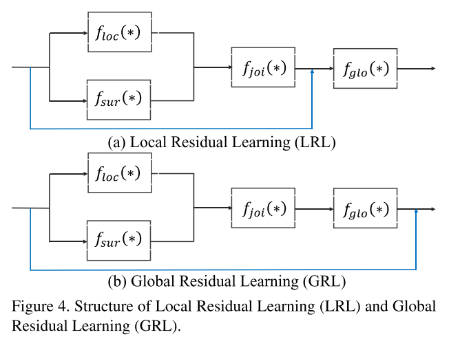
- 또한 CG 블록은 학습 시 성능 개선을 위하여 backpropagation 시 residual learning을 사용합니다. 제안된 CG 블록에는 두 가지 유형의 residual connection이 있습니다. 직관적으로 보았을 때, GRL이 LRL보다 네트워크에서 정보의 흐름에 더 큰 역할을 하는 것으로 생각 됩니다.
LRL(Local Residual Learning): input + joint featureGRL(Global Residual Learning): input + global feature
Context Guided Network
- 제안된 CG 블록을 기반으로, 파라미터 수를 줄이기 위해 CGNet의 구조를 정교하게 설계하였습니다. CGNet은 메모리 공간을 최대한 절약하기 위해 “깊고 얇게”라는 주요 원칙을 따릅니다.
- 특히 원작자가 제안한 CGNet 구조를 보면 51개의 컨벌루션 레이어만을 가지는데 이는 다른 모델에 비해서 상당히 얕은 레이어 수준입니다.
- 또한 공간 정보를 보다 잘 보존하기 위해 다운 샘플링 단계가 3단계에 불과하고 1/8 feature map resolution를 사용합니다. 이는 다른 많은 세그멘테이션 모델에서 사용하는 다운샘플링 5단계, feature map resolution가 1/32인 것과 차이가 있습니다.
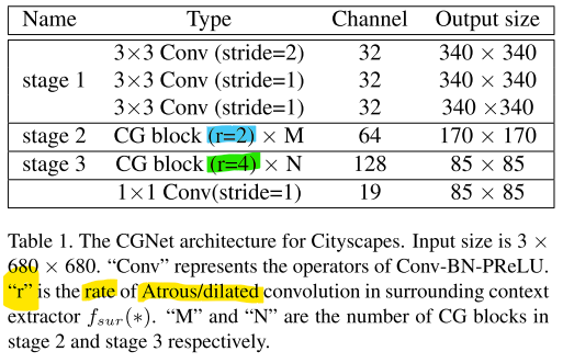
- 위 테이블에서는 CGNet의 상세 구조가 표현되어 있습니다. 아래 내용은 실제 코드에 구현된 컨셉들을 설명합니다. 글만 읽으면 다소 추상적일 수 있으니pytorch 코드와 비교하면서 읽어보시길 바랍니다.
- 1 단계에서는 standard convolution layer를 3개를 쌓아서 1/2 resolution의 feature map을 얻고, 2 단계와 3 단계에서는 각각 M개, N개의 CG 블록을 쌓아서 입력 이미지의 1/4, 1/8로 다운 샘플링한 feature map을 얻습니다. 코드는 다음과 같습니다. 코드의 클래스를 이용하여
stride = 2를 적용하면 resolution을 반으로 줄일 수 있습니다.
class ConvBNPReLU(nn.Module):
    def __init__(self, nIn, nOut, kSize, stride=1):
        """
        args:
            nIn: number of input channels
            nOut: number of output channels
            kSize: kernel size
            stride: stride rate for down-sampling. Default is 1
        """
        super().__init__()
        padding = int((kSize - 1)/2)
        self.conv = nn.Conv2d(nIn, nOut, (kSize, kSize), stride=stride, padding=(padding, padding), bias=False)
        self.bn = nn.BatchNorm2d(nOut, eps=1e-03)
        self.act = nn.PReLU(nOut)

    def forward(self, input):
        """
        args:
           input: input feature map
           return: transformed feature map
        """
        output = self.conv(input)
        output = self.bn(output)
        output = self.act(output)
        return output
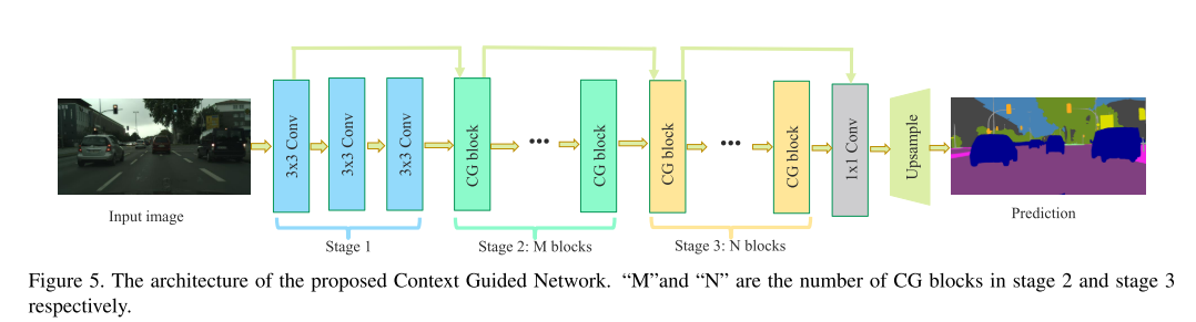
- 위 그림의 단계 별 화살표와 같이 2 단계와 3 단계에서는 이전 단계의 첫 번째 블록과 마지막 블록을 결합하여 첫 번째 계층의 입력을 얻음으로써 feature의 재사용과 더불어 residual learning을 할 수 있도록 합니다.
- CCNet의 정보 흐름을 개선하기 위해, 2단계와 3단계 각각 1/4 및 1/8의 다운 샘플링된 입력 영상을 추가로 전달하는 input injection 메커니즘을 취합니다. input injection 구조는 다음과 같습니다. Average Pooling을 이용하여 resolution을 downsamplingRatio = 1 이면 1/2로 줄이고 downsamplingRatio = 2이면 1/4로 줄이는 구조입니다.
class InputInjection(nn.Module):
    def __init__(self, downsamplingRatio):
        super().__init__()
        self.pool = nn.ModuleList()
        for i in range(0, downsamplingRatio):
            self.pool.append(nn.AvgPool2d(3, stride=2, padding=1))
    def forward(self, input):
        for pool in self.pool:
            input = pool(input)
        return input
- 2단계와 3단계의 모든 단위에 CG 블록이 사용된다는 것은 CGNet의 거의 모든 단계에서 CG 블록이 활용된다는 것을 의미합니다.
- 따라서, CGNet은 깊은 계층의
semantic level과 얕은 계층의spatial level모두에서 아래로부터 위까지 상황별 정보를 수집할 수 있는 기능을 가지고 있습니다. - 이는 인코딩 단계 이후 context module 을 수행하여 context 정보를 무시하거나 깊은 계층의 semantic level 에서 context 정보만 포착하는 기존의 세그멘테이션 모델과 비교하면 좀 더 세그멘테이션에 적합한 모델이라 할 수 있습니다.
- 또한, 매개변수의 수를 더욱 줄이기 위해 \(f_{loc}(*)\) 및 \(f_{sur}(*)\) 는 channel-wise convolution 을 채택하여 채널 간 계산 비용을 제거하고 메모리 공간을 많이 절약합니다.
Experiments
- 논문에서 제공하는 다양한 실험 결과들이 있습니다. 전체 실험 내용들은 논문을 참조하시기 바랍니다.
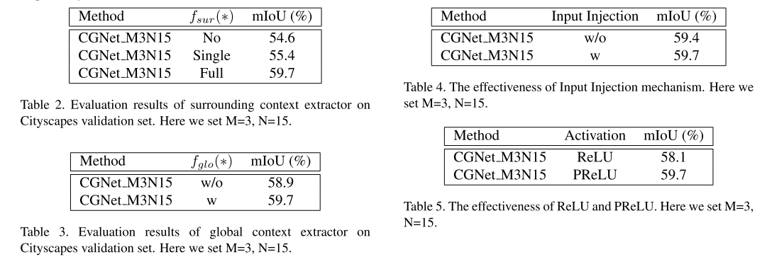
- 위 내용은 \(f_{sur}(*), f_{glo}(*)\), Input Injection, PReLU가 효과가 있음을 실험을 통해 확인합니다.
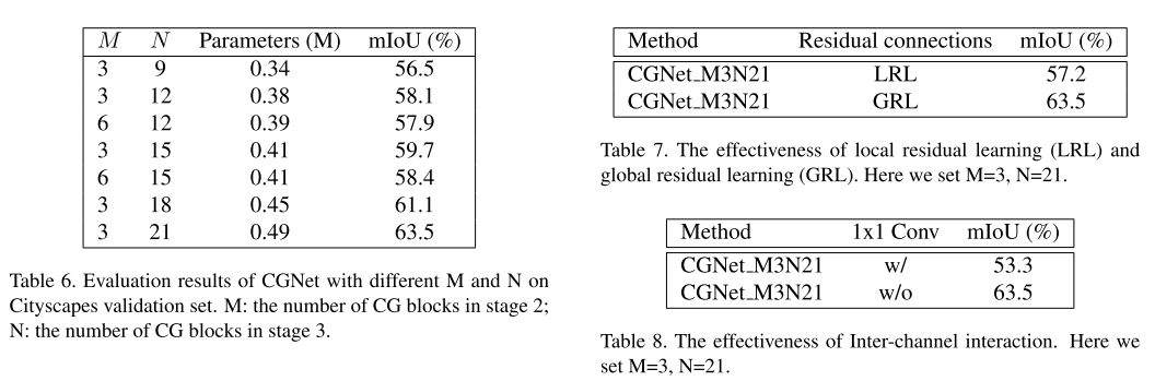
- 위 내용은 \(M, N\) 크기를 증가함에 따른 성능의 변화와, LRL, GRL의 효과 그리고 1x1 convolution의 효과에 대하여 실험을 통해 확인합니다.
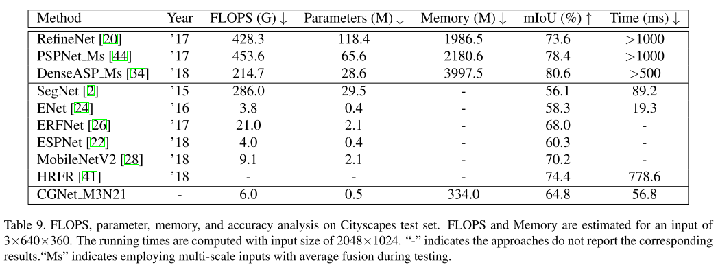
- 파라미터 \(M = 3, N = 21\)을 기준으로 다른 네트워크와 비교하였을 때, 실시간 세그멘테이션이 가능한 ENet, ESPNet에 비해 모든 면에서 우수하며 ERFNet에 비해서는 파라미터 갯수 대비 우수함을 보입니다.
Pytorch code
import torch
import torch.nn as nn
import torch.nn.functional as F

__all__ = ["Context_Guided_Network"]
#Filter out variables, functions, and classes that other programs don't need or don't want when running cmd "from CGNet import *"

class ConvBNPReLU(nn.Module):
    def __init__(self, nIn, nOut, kSize, stride=1):
        """
        args:
            nIn: number of input channels
            nOut: number of output channels
            kSize: kernel size
            stride: stride rate for down-sampling. Default is 1
        """
        super().__init__()
        padding = int((kSize - 1)/2)
        self.conv = nn.Conv2d(nIn, nOut, (kSize, kSize), stride=stride, padding=(padding, padding), bias=False)
        self.bn = nn.BatchNorm2d(nOut, eps=1e-03)
        self.act = nn.PReLU(nOut)

    def forward(self, input):
        """
        args:
           input: input feature map
           return: transformed feature map
        """
        output = self.conv(input)
        output = self.bn(output)
        output = self.act(output)
        return output


class BNPReLU(nn.Module):
    def __init__(self, nOut):
        """
        args:
           nOut: channels of output feature maps
        """
        super().__init__()
        self.bn = nn.BatchNorm2d(nOut, eps=1e-03)
        self.act = nn.PReLU(nOut)

    def forward(self, input):
        """
        args:
           input: input feature map
           return: normalized and thresholded feature map
        """
        output = self.bn(input)
        output = self.act(output)
        return output

class ConvBN(nn.Module):
    def __init__(self, nIn, nOut, kSize, stride=1):
        """
        args:
           nIn: number of input channels
           nOut: number of output channels
           kSize: kernel size
           stride: optinal stide for down-sampling
        """
        super().__init__()
        padding = int((kSize - 1)/2)
        self.conv = nn.Conv2d(nIn, nOut, (kSize, kSize), stride=stride, padding=(padding, padding), bias=False)
        self.bn = nn.BatchNorm2d(nOut, eps=1e-03)

    def forward(self, input):
        """
        args:
           input: input feature map
           return: transformed feature map
        """
        output = self.conv(input)
        output = self.bn(output)
        return output

class Conv(nn.Module):
    def __init__(self, nIn, nOut, kSize, stride=1):
        """
        args:
            nIn: number of input channels
            nOut: number of output channels
            kSize: kernel size
            stride: optional stride rate for down-sampling
        """
        super().__init__()
        padding = int((kSize - 1)/2)
        self.conv = nn.Conv2d(nIn, nOut, (kSize, kSize), stride=stride, padding=(padding, padding), bias=False)

    def forward(self, input):
        """
        args:
           input: input feature map
           return: transformed feature map
        """
        output = self.conv(input)
        return output

class ChannelWiseConv(nn.Module):
    def __init__(self, nIn, nOut, kSize, stride=1):
        """
        Args:
            nIn: number of input channels
            nOut: number of output channels, default (nIn == nOut)
            kSize: kernel size
            stride: optional stride rate for down-sampling
        """
        super().__init__()
        padding = int((kSize - 1)/2)
        self.conv = nn.Conv2d(nIn, nOut, (kSize, kSize), stride=stride, padding=(padding, padding), groups=nIn, bias=False)

    def forward(self, input):
        """
        args:
           input: input feature map
           return: transformed feature map
        """
        output = self.conv(input)
        return output

class DilatedConv(nn.Module):
    def __init__(self, nIn, nOut, kSize, stride=1, d=1):
        """
        args:
           nIn: number of input channels
           nOut: number of output channels
           kSize: kernel size
           stride: optional stride rate for down-sampling
           d: dilation rate
        """
        super().__init__()
        padding = int((kSize - 1)/2) * d
        self.conv = nn.Conv2d(nIn, nOut, (kSize, kSize), stride=stride, padding=(padding, padding), bias=False, dilation=d)

    def forward(self, input):
        """
        args:
           input: input feature map
           return: transformed feature map
        """
        output = self.conv(input)
        return output

class ChannelWiseDilatedConv(nn.Module):
    def __init__(self, nIn, nOut, kSize, stride=1, d=1):
        """
        args:
           nIn: number of input channels
           nOut: number of output channels, default (nIn == nOut)
           kSize: kernel size
           stride: optional stride rate for down-sampling
           d: dilation rate
        """
        super().__init__()
        padding = int((kSize - 1)/2) * d
        self.conv = nn.Conv2d(nIn, nOut, (kSize, kSize), stride=stride, padding=(padding, padding), groups= nIn, bias=False, dilation=d)

    def forward(self, input):
        """
        args:
           input: input feature map
           return: transformed feature map
        """
        output = self.conv(input)
        return output

class FGlo(nn.Module):
    """
    the FGlo class is employed to refine the joint feature of both local feature and surrounding context.
    """
    def __init__(self, channel, reduction=16):
        super(FGlo, self).__init__()
        self.avg_pool = nn.AdaptiveAvgPool2d(1)
        self.fc = nn.Sequential(
                nn.Linear(channel, channel // reduction),
                nn.ReLU(inplace=True),
                nn.Linear(channel // reduction, channel),
                nn.Sigmoid()
        )

    def forward(self, x):
        b, c, _, _ = x.size()
        y = self.avg_pool(x).view(b, c)
        y = self.fc(y).view(b, c, 1, 1)
        return x * y

class ContextGuidedBlock_Down(nn.Module):
    """
    the size of feature map divided 2, (H,W,C)---->(H/2, W/2, 2C)
    """
    def __init__(self, nIn, nOut, dilation_rate=2, reduction=16):
        """
        args:
           nIn: the channel of input feature map
           nOut: the channel of output feature map, and nOut=2*nIn
        """
        super().__init__()
        self.conv1x1 = ConvBNPReLU(nIn, nOut, 3, 2)  #  size/2, channel: nIn--->nOut

        self.F_loc = ChannelWiseConv(nOut, nOut, 3, 1)
        self.F_sur = ChannelWiseDilatedConv(nOut, nOut, 3, 1, dilation_rate)

        self.bn = nn.BatchNorm2d(2*nOut, eps=1e-3)
        self.act = nn.PReLU(2*nOut)
        self.reduce = Conv(2*nOut, nOut,1,1)  #reduce dimension: 2*nOut--->nOut

        self.F_glo = FGlo(nOut, reduction)

    def forward(self, input):
        output = self.conv1x1(input)
        loc = self.F_loc(output)
        sur = self.F_sur(output)

        joi_feat = torch.cat([loc, sur],1)  #  the joint feature
        joi_feat = self.bn(joi_feat)
        joi_feat = self.act(joi_feat)
        joi_feat = self.reduce(joi_feat)     #channel= nOut

        output = self.F_glo(joi_feat)  # F_glo is employed to refine the joint feature

        return output


class ContextGuidedBlock(nn.Module):
    def __init__(self, nIn, nOut, dilation_rate=2, reduction=16, add=True):
        """
        args:
           nIn: number of input channels
           nOut: number of output channels,
           add: if true, residual learning
        """
        super().__init__()
        n= int(nOut/2)
        self.conv1x1 = ConvBNPReLU(nIn, n, 1, 1)  #1x1 Conv is employed to reduce the computation
        self.F_loc = ChannelWiseConv(n, n, 3, 1) # local feature
        self.F_sur = ChannelWiseDilatedConv(n, n, 3, 1, dilation_rate) # surrounding context
        self.bn_prelu = BNPReLU(nOut)
        self.add = add
        self.F_glo= FGlo(nOut, reduction)

    def forward(self, input):
        output = self.conv1x1(input)
        loc = self.F_loc(output)
        sur = self.F_sur(output)

        joi_feat = torch.cat([loc, sur], 1)

        joi_feat = self.bn_prelu(joi_feat)

        output = self.F_glo(joi_feat)  #F_glo is employed to refine the joint feature
        # if residual version
        if self.add:
            output  = input + output
        return output

class InputInjection(nn.Module):
    def __init__(self, downsamplingRatio):
        super().__init__()
        self.pool = nn.ModuleList()
        for i in range(0, downsamplingRatio):
            self.pool.append(nn.AvgPool2d(3, stride=2, padding=1))
    def forward(self, input):
        for pool in self.pool:
            input = pool(input)
        return input


class Context_Guided_Network(nn.Module):
    """
    This class defines the proposed Context Guided Network (CGNet) in this work.
    """
    def __init__(self, classes=19, M= 3, N= 21, dropout_flag = False):
        """
        args:
          classes: number of classes in the dataset. Default is 19 for the cityscapes
          M: the number of blocks in stage 2
          N: the number of blocks in stage 3
        """
        super().__init__()
        self.level1_0 = ConvBNPReLU(3, 32, 3, 2)      # feature map size divided 2, 1/2
        self.level1_1 = ConvBNPReLU(32, 32, 3, 1)
        self.level1_2 = ConvBNPReLU(32, 32, 3, 1)

        self.sample1 = InputInjection(1)  #down-sample for Input Injection, factor=2
        self.sample2 = InputInjection(2)  #down-sample for Input Injiection, factor=4

        self.b1 = BNPReLU(32 + 3)

        #stage 2
        self.level2_0 = ContextGuidedBlock_Down(32 +3, 64, dilation_rate=2,reduction=8)
        self.level2 = nn.ModuleList()
        for i in range(0, M-1):
            self.level2.append(ContextGuidedBlock(64 , 64, dilation_rate=2, reduction=8))  #CG block
        self.bn_prelu_2 = BNPReLU(128 + 3)

        #stage 3
        self.level3_0 = ContextGuidedBlock_Down(128 + 3, 128, dilation_rate=4, reduction=16)
        self.level3 = nn.ModuleList()
        for i in range(0, N-1):
            self.level3.append(ContextGuidedBlock(128 , 128, dilation_rate=4, reduction=16)) # CG block
        self.bn_prelu_3 = BNPReLU(256)

        if dropout_flag:
            print("have droput layer")
            self.classifier = nn.Sequential(nn.Dropout2d(0.1, False),Conv(256, classes, 1, 1))
        else:
            self.classifier = nn.Sequential(Conv(256, classes, 1, 1))

        #init weights
        for m in self.modules():
            classname = m.__class__.__name__
            if classname.find('Conv2d')!= -1:
                nn.init.kaiming_normal_(m.weight)
                if m.bias is not None:
                    m.bias.data.zero_()
                elif classname.find('ConvTranspose2d')!= -1:
                    nn.init.kaiming_normal_(m.weight)
                    if m.bias is not None:
                        m.bias.data.zero_()

    def forward(self, input):
        """
        args:
            input: Receives the input RGB image
            return: segmentation map
        """
        # stage 1
        output0 = self.level1_0(input)
        output0 = self.level1_1(output0)
        output0 = self.level1_2(output0)
        inp1 = self.sample1(input)
        inp2 = self.sample2(input)

        # stage 2
        output0_cat = self.b1(torch.cat([output0, inp1], 1))
        output1_0 = self.level2_0(output0_cat) # down-sampled

        for i, layer in enumerate(self.level2):
            if i==0:
                output1 = layer(output1_0)
            else:
                output1 = layer(output1)

        output1_cat = self.bn_prelu_2(torch.cat([output1,  output1_0, inp2], 1))

        # stage 3
        output2_0 = self.level3_0(output1_cat) # down-sampled
        for i, layer in enumerate(self.level3):
            if i==0:
                output2 = layer(output2_0)
            else:
                output2 = layer(output2)

        output2_cat = self.bn_prelu_3(torch.cat([output2_0, output2], 1))

        # classifier
        classifier = self.classifier(output2_cat)

        # upsample segmenation map ---> the input image size
        out = F.upsample(classifier, input.size()[2:], mode='bilinear',align_corners = False)   #Upsample score map, factor=8
        return out